Testing Linear Regression Assumptions in Python

Checking model assumptions is like commenting code. Everybody should be doing it often, but it sometimes ends up being overlooked in reality. A failure to do either can result in a lot of time being confused, going down rabbit holes, and can have pretty serious consequences from the model not being interpreted correctly.

Linear regression is a fundamental tool that has distinct advantages over other regression algorithms. Due to its simplicity, it’s an exceptionally quick algorithm to train, thus typically makes it a good baseline algorithm for common regression scenarios. More importantly, models trained with linear regression are the most interpretable kind of regression models available - meaning it’s easier to take action from the results of a linear regression model. However, if the assumptions are not satisfied, the interpretation of the results will not always be valid. This can be very dangerous depending on the application.

This post contains code for tests on the assumptions of linear regression and examples with both a real-world dataset and a toy dataset.

The Data

For our real-world dataset, we’ll use the Boston house prices dataset from the late 1970’s. The toy dataset will be created using scikit-learn’s make_regression function which creates a dataset that should perfectly satisfy all of our assumptions.

One thing to note is that I’m assuming outliers have been removed in this blog post. This is an important part of any exploratory data analysis (which isn’t being performed in this post in order to keep it short) that should happen in real world scenarios, and outliers in particular will cause significant issues with linear regression. See Anscombe’s Quartet for examples of outliers causing issues with fitting linear regression models.

Here are the variable descriptions for the Boston housing dataset straight from the documentation:

• CRIM: Per capita crime rate by town

• ZN: Proportion of residential land zoned for lots over 25,000 sq.ft.

• INDUS: Proportion of non-retail business acres per town.

• CHAS: Charles River dummy variable (1 if tract bounds river; 0 otherwise)

• NOX: Nitric oxides concentration (parts per 10 million)

• RM: Average number of rooms per dwelling

• AGE: Proportion of owner-occupied units built prior to 1940

• DIS: Weighted distances to five Boston employment centers

• RAD: Index of accessibility to radial highways

• TAX: Full-value property-tax rate per $10,000

• PTRATIO: Pupil-teacher ratio by town

• B: 1000(Bk - 0.63)^2 where Bk is the proportion of blacks by town

  • Note: I really don’t like this variable because I think it’s both highly unethical to determine house prices by the color of people’s skin in a given area in a predictive modeling scenario and it irks me that it singles out one ethnicity rather than including all others. I am leaving it in for this post to keep the code simple, but I would remove it in a real-world situation.

• LSTAT: % lower status of the population

• MEDV: Median value of owner-occupied homes in $1,000’s

import numpy as np
import pandas as pd
import matplotlib.pyplot as plt
import seaborn as sns
from sklearn import datasets
%matplotlib inline


"""
Real-world data of Boston housing prices
Additional Documentation: https://www.cs.toronto.edu/~delve/data/boston/bostonDetail.html

Attributes:
data: Features/predictors
label: Target/label/response variable
feature_names: Abbreviations of names of features
"""
boston = datasets.load_boston()


"""
Artificial linear data using the same number of features and observations as the
Boston housing prices dataset for assumption test comparison
"""
linear_X, linear_y = datasets.make_regression(n_samples=boston.data.shape[0],
                                              n_features=boston.data.shape[1],
                                              noise=75, random_state=46)

# Setting feature names to x1, x2, x3, etc. if they are not defined
linear_feature_names = ['X'+str(feature+1) for feature in range(linear_X.shape[1])]

Now that the data is loaded in, let’s preview it:

df = pd.DataFrame(boston.data, columns=boston.feature_names)
df['HousePrice'] = boston.target

df.head()

	CRIM	ZN	INDUS	CHAS	NOX	RM	AGE	DIS	RAD	TAX	PTRATIO	B	LSTAT	HousePrice
0	0.00632	18.0	2.31	0.0	0.538	6.575	65.2	4.0900	1.0	296.0	15.3	396.90	4.98	24.0
1	0.02731	0.0	7.07	0.0	0.469	6.421	78.9	4.9671	2.0	242.0	17.8	396.90	9.14	21.6
2	0.02729	0.0	7.07	0.0	0.469	7.185	61.1	4.9671	2.0	242.0	17.8	392.83	4.03	34.7
3	0.03237	0.0	2.18	0.0	0.458	6.998	45.8	6.0622	3.0	222.0	18.7	394.63	2.94	33.4
4	0.06905	0.0	2.18	0.0	0.458	7.147	54.2	6.0622	3.0	222.0	18.7	396.90	5.33	36.2

Initial Setup

Before we test the assumptions, we’ll need to fit our linear regression models. I have a master function for performing all of the assumption testing at the bottom of this post that does this automatically, but to abstract the assumption tests out to view them independently we’ll have to re-write the individual tests to take the trained model as a parameter.

Additionally, a few of the tests use residuals, so we’ll write a quick function to calculate residuals. These are also calculated once in the master function at the bottom of the page, but this extra function is to adhere to DRY typing for the individual tests that use residuals.

from sklearn.linear_model import LinearRegression

# Fitting the model
boston_model = LinearRegression()
boston_model.fit(boston.data, boston.target)

# Returning the R^2 for the model
boston_r2 = boston_model.score(boston.data, boston.target)
print('R^2: {0}'.format(boston_r2))

R^2: 0.7406077428649428

# Fitting the model
linear_model = LinearRegression()
linear_model.fit(linear_X, linear_y)

# Returning the R^2 for the model
linear_r2 = linear_model.score(linear_X, linear_y)
print('R^2: {0}'.format(linear_r2))

R^2: 0.873743725796525

def calculate_residuals(model, features, label):
    """
    Creates predictions on the features with the model and calculates residuals
    """
    predictions = model.predict(features)
    df_results = pd.DataFrame({'Actual': label, 'Predicted': predictions})
    df_results['Residuals'] = abs(df_results['Actual']) - abs(df_results['Predicted'])
    
    return df_results

We’re all set, so onto the assumption testing!

Assumptions

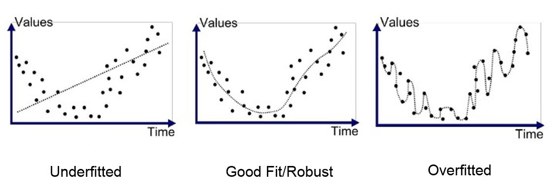
I) Linearity

This assumes that there is a linear relationship between the predictors (e.g. independent variables or features) and the response variable (e.g. dependent variable or label). This also assumes that the predictors are additive.

Why it can happen: There may not just be a linear relationship among the data. Modeling is about trying to estimate a function that explains a process, and linear regression would not be a fitting estimator (pun intended) if there is no linear relationship.

What it will affect: The predictions will be extremely inaccurate because our model is underfitting. This is a serious violation that should not be ignored.

How to detect it: If there is only one predictor, this is pretty easy to test with a scatter plot. Most cases aren’t so simple, so we’ll have to modify this by using a scatter plot to see our predicted values versus the actual values (in other words, view the residuals). Ideally, the points should lie on or around a diagonal line on the scatter plot.

How to fix it: Either adding polynomial terms to some of the predictors or applying nonlinear transformations . If those do not work, try adding additional variables to help capture the relationship between the predictors and the label.

def linear_assumption(model, features, label):
    """
    Linearity: Assumes that there is a linear relationship between the predictors and
               the response variable. If not, either a quadratic term or another
               algorithm should be used.
    """
    print('Assumption 1: Linear Relationship between the Target and the Feature', '\n')
        
    print('Checking with a scatter plot of actual vs. predicted.',
           'Predictions should follow the diagonal line.')
    
    # Calculating residuals for the plot
    df_results = calculate_residuals(model, features, label)
    
    # Plotting the actual vs predicted values
    sns.lmplot(x='Actual', y='Predicted', data=df_results, fit_reg=False, size=7)
        
    # Plotting the diagonal line
    line_coords = np.arange(df_results.min().min(), df_results.max().max())
    plt.plot(line_coords, line_coords,  # X and y points
             color='darkorange', linestyle='--')
    plt.title('Actual vs. Predicted')
    plt.show()

We’ll start with our linear dataset:

linear_assumption(linear_model, linear_X, linear_y)

Assumption 1: Linear Relationship between the Target and the Feature

Checking with a scatter plot of actual vs. predicted. Predictions should follow the diagonal line.

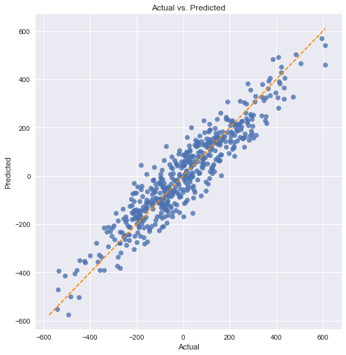
We can see a relatively even spread around the diagonal line.

Now, let’s compare it to the Boston dataset:

linear_assumption(boston_model, boston.data, boston.target)

Assumption 1: Linear Relationship between the Target and the Feature

Checking with a scatter plot of actual vs. predicted. Predictions should follow the diagonal line.

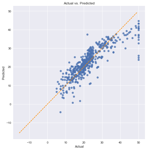
We can see in this case that there is not a perfect linear relationship. Our predictions are biased towards lower values in both the lower end (around 5-10) and especially at the higher values (above 40).

II) Normality of the Error Terms

More specifically, this assumes that the error terms of the model are normally distributed. Linear regressions other than Ordinary Least Squares (OLS) may also assume normality of the predictors or the label, but that is not the case here.

Why it can happen: This can actually happen if either the predictors or the label are significantly non-normal. Other potential reasons could include the linearity assumption being violated or outliers affecting our model.

What it will affect: A violation of this assumption could cause issues with either shrinking or inflating our confidence intervals.

How to detect it: There are a variety of ways to do so, but we’ll look at both a histogram and the p-value from the Anderson-Darling test for normality.

How to fix it: It depends on the root cause, but there are a few options. Nonlinear transformations of the variables, excluding specific variables (such as long-tailed variables), or removing outliers may solve this problem.

def normal_errors_assumption(model, features, label, p_value_thresh=0.05):
    """
    Normality: Assumes that the error terms are normally distributed. If they are not,
    nonlinear transformations of variables may solve this.
               
    This assumption being violated primarily causes issues with the confidence intervals
    """
    from statsmodels.stats.diagnostic import normal_ad
    print('Assumption 2: The error terms are normally distributed', '\n')
    
    # Calculating residuals for the Anderson-Darling test
    df_results = calculate_residuals(model, features, label)
    
    print('Using the Anderson-Darling test for normal distribution')

    # Performing the test on the residuals
    p_value = normal_ad(df_results['Residuals'])[1]
    print('p-value from the test - below 0.05 generally means non-normal:', p_value)
    
    # Reporting the normality of the residuals
    if p_value < p_value_thresh:
        print('Residuals are not normally distributed')
    else:
        print('Residuals are normally distributed')
    
    # Plotting the residuals distribution
    plt.subplots(figsize=(12, 6))
    plt.title('Distribution of Residuals')
    sns.distplot(df_results['Residuals'])
    plt.show()
    
    print()
    if p_value > p_value_thresh:
        print('Assumption satisfied')
    else:
        print('Assumption not satisfied')
        print()
        print('Confidence intervals will likely be affected')
        print('Try performing nonlinear transformations on variables')

As with our previous assumption, we’ll start with the linear dataset:

normal_errors_assumption(linear_model, linear_X, linear_y)

Assumption 2: The error terms are normally distributed

Using the Anderson-Darling test for normal distribution
p-value from the test - below 0.05 generally means non-normal: 0.335066045847
Residuals are normally distributed

Assumption satisfied

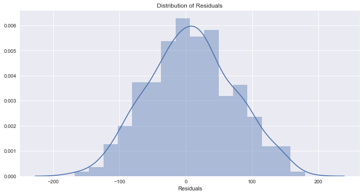
Now let’s run the same test on the Boston dataset:

normal_errors_assumption(boston_model, boston.data, boston.target)

Assumption 2: The error terms are normally distributed

Using the Anderson-Darling test for normal distribution
p-value from the test - below 0.05 generally means non-normal: 7.78748286642e-25
Residuals are not normally distributed

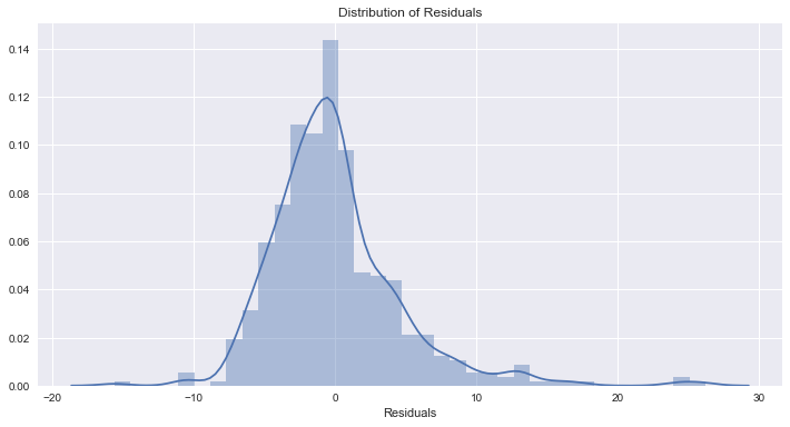
Assumption not satisfied

Confidence intervals will likely be affected
Try performing nonlinear transformations on variables

This isn’t ideal, and we can see that our model is biasing towards under-estimating.

III) No Multicollinearity among Predictors

This assumes that the predictors used in the regression are not correlated with each other. This won’t render our model unusable if violated, but it will cause issues with the interpretability of the model.

Why it can happen: A lot of data is just naturally correlated. For example, if trying to predict a house price with square footage, the number of bedrooms, and the number of bathrooms, we can expect to see correlation between those three variables because bedrooms and bathrooms make up a portion of square footage.

What it will affect: Multicollinearity causes issues with the interpretation of the coefficients. Specifically, you can interpret a coefficient as “an increase of 1 in this predictor results in a change of (coefficient) in the response variable, holding all other predictors constant.” This becomes problematic when multicollinearity is present because we can’t hold correlated predictors constant. Additionally, it increases the standard error of the coefficients, which results in them potentially showing as statistically insignificant when they might actually be significant.

How to detect it: There are a few ways, but we will use a heatmap of the correlation as a visual aid and examine the variance inflation factor (VIF).

How to fix it: This can be fixed by other removing predictors with a high variance inflation factor (VIF) or performing dimensionality reduction.

def multicollinearity_assumption(model, features, label, feature_names=None):
    """
    Multicollinearity: Assumes that predictors are not correlated with each other. If there is
                       correlation among the predictors, then either remove prepdictors with high
                       Variance Inflation Factor (VIF) values or perform dimensionality reduction
                           
                       This assumption being violated causes issues with interpretability of the 
                       coefficients and the standard errors of the coefficients.
    """
    from statsmodels.stats.outliers_influence import variance_inflation_factor
    print('Assumption 3: Little to no multicollinearity among predictors')
        
    # Plotting the heatmap
    plt.figure(figsize = (10,8))
    sns.heatmap(pd.DataFrame(features, columns=feature_names).corr(), annot=True)
    plt.title('Correlation of Variables')
    plt.show()
        
    print('Variance Inflation Factors (VIF)')
    print('> 10: An indication that multicollinearity may be present')
    print('> 100: Certain multicollinearity among the variables')
    print('-------------------------------------')
       
    # Gathering the VIF for each variable
    VIF = [variance_inflation_factor(features, i) for i in range(features.shape[1])]
    for idx, vif in enumerate(VIF):
        print('{0}: {1}'.format(feature_names[idx], vif))
        
    # Gathering and printing total cases of possible or definite multicollinearity
    possible_multicollinearity = sum([1 for vif in VIF if vif > 10])
    definite_multicollinearity = sum([1 for vif in VIF if vif > 100])
    print()
    print('{0} cases of possible multicollinearity'.format(possible_multicollinearity))
    print('{0} cases of definite multicollinearity'.format(definite_multicollinearity))
    print()

    if definite_multicollinearity == 0:
        if possible_multicollinearity == 0:
            print('Assumption satisfied')
        else:
            print('Assumption possibly satisfied')
            print()
            print('Coefficient interpretability may be problematic')
            print('Consider removing variables with a high Variance Inflation Factor (VIF)')

    else:
        print('Assumption not satisfied')
        print()
        print('Coefficient interpretability will be problematic')
        print('Consider removing variables with a high Variance Inflation Factor (VIF)')

Starting with the linear dataset:

multicollinearity_assumption(linear_model, linear_X, linear_y, linear_feature_names)

Assumption 3: Little to no multicollinearity among predictors

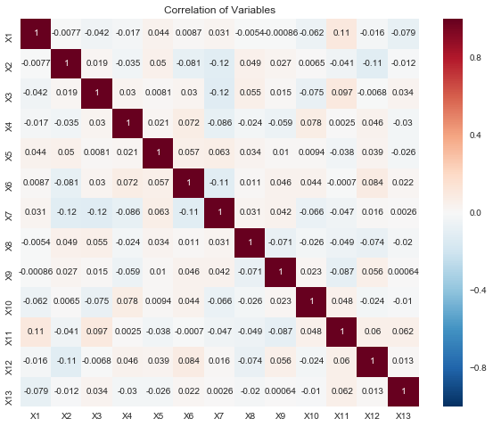
Variance Inflation Factors (VIF)
> 10: An indication that multicollinearity may be present
> 100: Certain multicollinearity among the variables
-------------------------------------
X1: 1.030931170297102
X2: 1.0457176802992108
X3: 1.0418076962011933
X4: 1.0269600632251443
X5: 1.0199882018822783
X6: 1.0404194675991594
X7: 1.0670847781889177
X8: 1.0229686036798158
X9: 1.0292923730360835
X10: 1.0289003332516535
X11: 1.052043220821624
X12: 1.0336719449364813
X13: 1.0140788728975834

0 cases of possible multicollinearity
0 cases of definite multicollinearity

Assumption satisfied

Everything looks peachy keen. Onto the Boston dataset:

multicollinearity_assumption(boston_model, boston.data, boston.target, boston.feature_names)

Assumption 3: Little to no multicollinearity among predictors

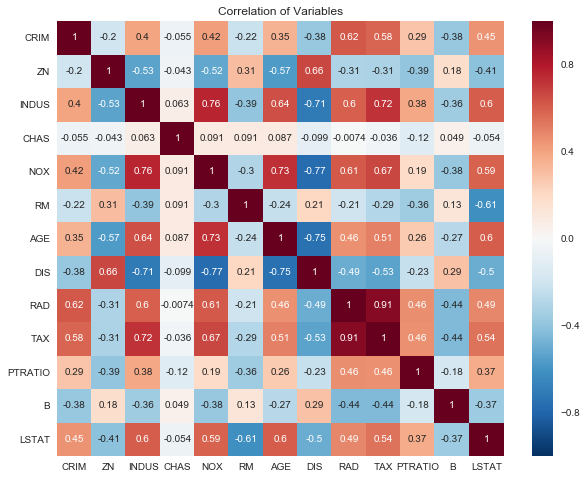
Variance Inflation Factors (VIF)
> 10: An indication that multicollinearity may be present
> 100: Certain multicollinearity among the variables
-------------------------------------
CRIM: 2.0746257632525675
ZN: 2.8438903527570782
INDUS: 14.484283435031545
CHAS: 1.1528909172683364
NOX: 73.90221170812129
RM: 77.93496867181426
AGE: 21.38677358304778
DIS: 14.699368125642422
RAD: 15.154741587164747
TAX: 61.226929320337554
PTRATIO: 85.0273135204276
B: 20.066007061121244
LSTAT: 11.088865100659874

10 cases of possible multicollinearity
0 cases of definite multicollinearity

Assumption possibly satisfied

Coefficient interpretability may be problematic
Consider removing variables with a high Variance Inflation Factor (VIF)

This isn’t quite as egregious as our normality assumption violation, but there is possible multicollinearity for most of the variables in this dataset.

IV) No Autocorrelation of the Error Terms

This assumes no autocorrelation of the error terms. Autocorrelation being present typically indicates that we are missing some information that should be captured by the model.

Why it can happen: In a time series scenario, there could be information about the past that we aren’t capturing. In a non-time series scenario, our model could be systematically biased by either under or over predicting in certain conditions. Lastly, this could be a result of a violation of the linearity assumption.

What it will affect: This will impact our model estimates.

How to detect it: We will perform a Durbin-Watson test to determine if either positive or negative correlation is present. Alternatively, you could create plots of residual autocorrelations.

How to fix it: A simple fix of adding lag variables can fix this problem. Alternatively, interaction terms, additional variables, or additional transformations may fix this.

def autocorrelation_assumption(model, features, label):
    """
    Autocorrelation: Assumes that there is no autocorrelation in the residuals. If there is
                     autocorrelation, then there is a pattern that is not explained due to
                     the current value being dependent on the previous value.
                     This may be resolved by adding a lag variable of either the dependent
                     variable or some of the predictors.
    """
    from statsmodels.stats.stattools import durbin_watson
    print('Assumption 4: No Autocorrelation', '\n')
    
    # Calculating residuals for the Durbin Watson-tests
    df_results = calculate_residuals(model, features, label)

    print('\nPerforming Durbin-Watson Test')
    print('Values of 1.5 < d < 2.5 generally show that there is no autocorrelation in the data')
    print('0 to 2< is positive autocorrelation')
    print('>2 to 4 is negative autocorrelation')
    print('-------------------------------------')
    durbinWatson = durbin_watson(df_results['Residuals'])
    print('Durbin-Watson:', durbinWatson)
    if durbinWatson < 1.5:
        print('Signs of positive autocorrelation', '\n')
        print('Assumption not satisfied')
    elif durbinWatson > 2.5:
        print('Signs of negative autocorrelation', '\n')
        print('Assumption not satisfied')
    else:
        print('Little to no autocorrelation', '\n')
        print('Assumption satisfied')

Testing with our ideal dataset:

autocorrelation_assumption(linear_model, linear_X, linear_y)

Assumption 4: No Autocorrelation


Performing Durbin-Watson Test
Values of 1.5 < d < 2.5 generally show that there is no autocorrelation in the data
0 to 2< is positive autocorrelation
>2 to 4 is negative autocorrelation
-------------------------------------
Durbin-Watson: 2.00345051385
Little to no autocorrelation

Assumption satisfied

And with our Boston dataset:

autocorrelation_assumption(boston_model, boston.data, boston.target)

Assumption 4: No Autocorrelation


Performing Durbin-Watson Test
Values of 1.5 < d < 2.5 generally show that there is no autocorrelation in the data
0 to 2< is positive autocorrelation
>2 to 4 is negative autocorrelation
-------------------------------------
Durbin-Watson: 1.0713285604
Signs of positive autocorrelation

Assumption not satisfied

We’re having signs of positive autocorrelation here, but we should expect this since we know our model is consistently under-predicting and our linearity assumption is being violated. Since this isn’t a time series dataset, lag variables aren’t possible. Instead, we should look into either interaction terms or additional transformations.

V) Homoscedasticity

This assumes homoscedasticity, which is the same variance within our error terms. Heteroscedasticity, the violation of homoscedasticity, occurs when we don’t have an even variance across the error terms.

Why it can happen: Our model may be giving too much weight to a subset of the data, particularly where the error variance was the largest.

What it will affect: Significance tests for coefficients due to the standard errors being biased. Additionally, the confidence intervals will be either too wide or too narrow.

How to detect it: Plot the residuals and see if the variance appears to be uniform.

How to fix it: Heteroscedasticity (can you tell I like the scedasticity words?) can be solved either by using weighted least squares regression instead of the standard OLS or transforming either the dependent or highly skewed variables. Performing a log transformation on the dependent variable is not a bad place to start.

def homoscedasticity_assumption(model, features, label):
    """
    Homoscedasticity: Assumes that the errors exhibit constant variance
    """
    print('Assumption 5: Homoscedasticity of Error Terms', '\n')
    
    print('Residuals should have relative constant variance')
        
    # Calculating residuals for the plot
    df_results = calculate_residuals(model, features, label)

    # Plotting the residuals
    plt.subplots(figsize=(12, 6))
    ax = plt.subplot(111)  # To remove spines
    plt.scatter(x=df_results.index, y=df_results.Residuals, alpha=0.5)
    plt.plot(np.repeat(0, df_results.index.max()), color='darkorange', linestyle='--')
    ax.spines['right'].set_visible(False)  # Removing the right spine
    ax.spines['top'].set_visible(False)  # Removing the top spine
    plt.title('Residuals')
    plt.show()  

Plotting the residuals of our ideal dataset:

homoscedasticity_assumption(linear_model, linear_X, linear_y)

Assumption 5: Homoscedasticity of Error Terms

Residuals should have relative constant variance

There don’t appear to be any obvious problems with that.

Next, looking at the residuals of the Boston dataset:

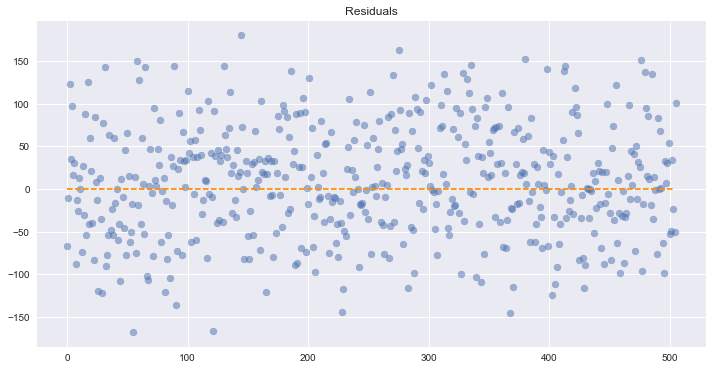
homoscedasticity_assumption(boston_model, boston.data, boston.target)

Assumption 5: Homoscedasticity of Error Terms

Residuals should have relative constant variance

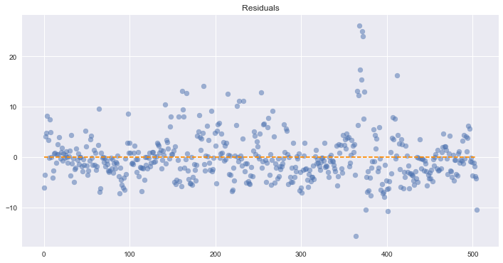
We can’t see a fully uniform variance across our residuals, so this is potentially problematic. However, we know from our other tests that our model has several issues and is under predicting in many cases.

Conclusion

We can clearly see that a linear regression model on the Boston dataset violates a number of assumptions which cause significant problems with the interpretation of the model itself. It’s not uncommon for assumptions to be violated on real-world data, but it’s important to check them so we can either fix them and/or be aware of the flaws in the model for the presentation of the results or the decision making process.

It is dangerous to make decisions on a model that has violated assumptions because those decisions are effectively being formulated on made-up numbers. Not only that, but it also provides a false sense of security due to trying to be empirical in the decision making process. Empiricism requires due diligence, which is why these assumptions exist and are stated up front. Hopefully this code can help ease the due diligence process and make it less painful.

Code for the Master Function

This function performs all of the assumption tests listed in this blog post:

def linear_regression_assumptions(features, label, feature_names=None):
    """
    Tests a linear regression on the model to see if assumptions are being met
    """
    from sklearn.linear_model import LinearRegression
    
    # Setting feature names to x1, x2, x3, etc. if they are not defined
    if feature_names is None:
        feature_names = ['X'+str(feature+1) for feature in range(features.shape[1])]
    
    print('Fitting linear regression')
    # Multi-threading if the dataset is a size where doing so is beneficial
    if features.shape[0] < 100000:
        model = LinearRegression(n_jobs=-1)
    else:
        model = LinearRegression()
        
    model.fit(features, label)
    
    # Returning linear regression R^2 and coefficients before performing diagnostics
    r2 = model.score(features, label)
    print()
    print('R^2:', r2, '\n')
    print('Coefficients')
    print('-------------------------------------')
    print('Intercept:', model.intercept_)
    
    for feature in range(len(model.coef_)):
        print('{0}: {1}'.format(feature_names[feature], model.coef_[feature]))

    print('\nPerforming linear regression assumption testing')
    
    # Creating predictions and calculating residuals for assumption tests
    predictions = model.predict(features)
    df_results = pd.DataFrame({'Actual': label, 'Predicted': predictions})
    df_results['Residuals'] = abs(df_results['Actual']) - abs(df_results['Predicted'])

    
    def linear_assumption():
        """
        Linearity: Assumes there is a linear relationship between the predictors and
                   the response variable. If not, either a polynomial term or another
                   algorithm should be used.
        """
        print('\n=======================================================================================')
        print('Assumption 1: Linear Relationship between the Target and the Features')
        
        print('Checking with a scatter plot of actual vs. predicted. Predictions should follow the diagonal line.')
        
        # Plotting the actual vs predicted values
        sns.lmplot(x='Actual', y='Predicted', data=df_results, fit_reg=False, size=7)
        
        # Plotting the diagonal line
        line_coords = np.arange(df_results.min().min(), df_results.max().max())
        plt.plot(line_coords, line_coords,  # X and y points
                 color='darkorange', linestyle='--')
        plt.title('Actual vs. Predicted')
        plt.show()
        print('If non-linearity is apparent, consider adding a polynomial term')
        
        
    def normal_errors_assumption(p_value_thresh=0.05):
        """
        Normality: Assumes that the error terms are normally distributed. If they are not,
        nonlinear transformations of variables may solve this.
               
        This assumption being violated primarily causes issues with the confidence intervals
        """
        from statsmodels.stats.diagnostic import normal_ad
        print('\n=======================================================================================')
        print('Assumption 2: The error terms are normally distributed')
        print()
    
        print('Using the Anderson-Darling test for normal distribution')

        # Performing the test on the residuals
        p_value = normal_ad(df_results['Residuals'])[1]
        print('p-value from the test - below 0.05 generally means non-normal:', p_value)
    
        # Reporting the normality of the residuals
        if p_value < p_value_thresh:
            print('Residuals are not normally distributed')
        else:
            print('Residuals are normally distributed')
    
        # Plotting the residuals distribution
        plt.subplots(figsize=(12, 6))
        plt.title('Distribution of Residuals')
        sns.distplot(df_results['Residuals'])
        plt.show()
    
        print()
        if p_value > p_value_thresh:
            print('Assumption satisfied')
        else:
            print('Assumption not satisfied')
            print()
            print('Confidence intervals will likely be affected')
            print('Try performing nonlinear transformations on variables')
        
        
    def multicollinearity_assumption():
        """
        Multicollinearity: Assumes that predictors are not correlated with each other. If there is
                           correlation among the predictors, then either remove prepdictors with high
                           Variance Inflation Factor (VIF) values or perform dimensionality reduction
                           
                           This assumption being violated causes issues with interpretability of the 
                           coefficients and the standard errors of the coefficients.
        """
        from statsmodels.stats.outliers_influence import variance_inflation_factor
        print('\n=======================================================================================')
        print('Assumption 3: Little to no multicollinearity among predictors')
        
        # Plotting the heatmap
        plt.figure(figsize = (10,8))
        sns.heatmap(pd.DataFrame(features, columns=feature_names).corr(), annot=True)
        plt.title('Correlation of Variables')
        plt.show()
        
        print('Variance Inflation Factors (VIF)')
        print('> 10: An indication that multicollinearity may be present')
        print('> 100: Certain multicollinearity among the variables')
        print('-------------------------------------')
       
        # Gathering the VIF for each variable
        VIF = [variance_inflation_factor(features, i) for i in range(features.shape[1])]
        for idx, vif in enumerate(VIF):
            print('{0}: {1}'.format(feature_names[idx], vif))
        
        # Gathering and printing total cases of possible or definite multicollinearity
        possible_multicollinearity = sum([1 for vif in VIF if vif > 10])
        definite_multicollinearity = sum([1 for vif in VIF if vif > 100])
        print()
        print('{0} cases of possible multicollinearity'.format(possible_multicollinearity))
        print('{0} cases of definite multicollinearity'.format(definite_multicollinearity))
        print()

        if definite_multicollinearity == 0:
            if possible_multicollinearity == 0:
                print('Assumption satisfied')
            else:
                print('Assumption possibly satisfied')
                print()
                print('Coefficient interpretability may be problematic')
                print('Consider removing variables with a high Variance Inflation Factor (VIF)')
        else:
            print('Assumption not satisfied')
            print()
            print('Coefficient interpretability will be problematic')
            print('Consider removing variables with a high Variance Inflation Factor (VIF)')
        
        
    def autocorrelation_assumption():
        """
        Autocorrelation: Assumes that there is no autocorrelation in the residuals. If there is
                         autocorrelation, then there is a pattern that is not explained due to
                         the current value being dependent on the previous value.
                         This may be resolved by adding a lag variable of either the dependent
                         variable or some of the predictors.
        """
        from statsmodels.stats.stattools import durbin_watson
        print('\n=======================================================================================')
        print('Assumption 4: No Autocorrelation')
        print('\nPerforming Durbin-Watson Test')
        print('Values of 1.5 < d < 2.5 generally show that there is no autocorrelation in the data')
        print('0 to 2< is positive autocorrelation')
        print('>2 to 4 is negative autocorrelation')
        print('-------------------------------------')
        durbinWatson = durbin_watson(df_results['Residuals'])
        print('Durbin-Watson:', durbinWatson)
        if durbinWatson < 1.5:
            print('Signs of positive autocorrelation', '\n')
            print('Assumption not satisfied', '\n')
            print('Consider adding lag variables')
        elif durbinWatson > 2.5:
            print('Signs of negative autocorrelation', '\n')
            print('Assumption not satisfied', '\n')
            print('Consider adding lag variables')
        else:
            print('Little to no autocorrelation', '\n')
            print('Assumption satisfied')

            
    def homoscedasticity_assumption():
        """
        Homoscedasticity: Assumes that the errors exhibit constant variance
        """
        print('\n=======================================================================================')
        print('Assumption 5: Homoscedasticity of Error Terms')
        print('Residuals should have relative constant variance')
        
        # Plotting the residuals
        plt.subplots(figsize=(12, 6))
        ax = plt.subplot(111)  # To remove spines
        plt.scatter(x=df_results.index, y=df_results.Residuals, alpha=0.5)
        plt.plot(np.repeat(0, df_results.index.max()), color='darkorange', linestyle='--')
        ax.spines['right'].set_visible(False)  # Removing the right spine
        ax.spines['top'].set_visible(False)  # Removing the top spine
        plt.title('Residuals')
        plt.show() 
        print('If heteroscedasticity is apparent, confidence intervals and predictions will be affected')
        
        
    linear_assumption()
    normal_errors_assumption()
    multicollinearity_assumption()
    autocorrelation_assumption()
    homoscedasticity_assumption()