
Competition: Analyze This! AI Innovation Challenge
Introduction
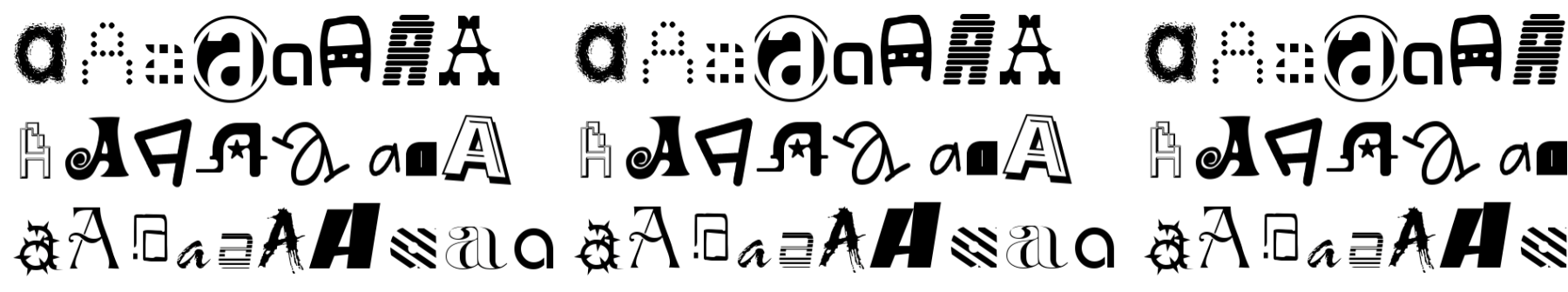
A few months ago, the twin cities meetup group Analyze This! hosted a competition on something rare in the area - deep learning. More specifically, the competition was on image classification of Yaroslav Bulatov’s notMNIST dataset (a few samples pictured in the header photo). This dataset is very similar to Yann LeCun’s MNIST dataset of handwritten digits, the “Iris dataset of deep learning”, but with less structure and more noise.
The script is at the bottom of the page, and here is a brief overview and explanation of what I did for this competition.
Methodology
For this competition, I prototyped different neural network architectures in Keras due to the ability of quickly creating and modifying architectures without worrying about things like graphs, sessions, weights, or placeholder variables. Since the competition required submissions to be done in TensorFlow, I re-created the best performing architecture in TensorFlow after finishing testing in Keras.
Data Preparation
Normalizing
In most cases, you need to normalize your inputs before feeding them to a neural network. This allows it to train faster, reduces the chances of getting stuck in a local optima, and provides a few other nice mathematical properties.
You will notice that there is no scaling or normalizing in the script. This is because it was already performed on the data that we are reading in.
Data Augmentation
Since our samples vary greatly within class, I wanted to produce additional training samples to help our network further learn and generalize. I initially looked into generative adversarial networks (GANs) to generate new training samples. This works by pitting two networks, a generator to generate the images from random noise and a discriminator to detect the fake images, against each other in order to cause the generator to become good enough at creating fake images that it can fool the discriminator:
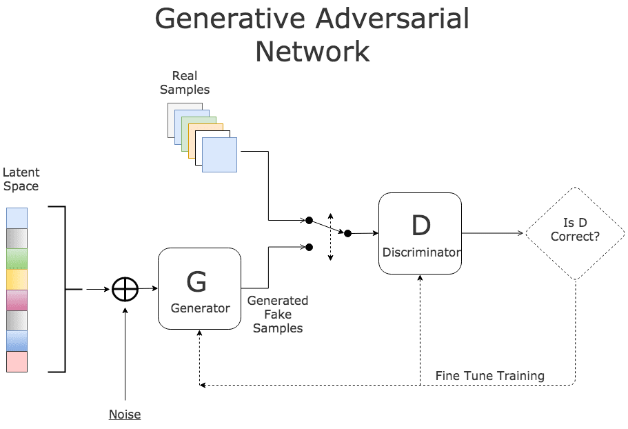
This is a very popular concept today, and I agree that it’s extremely interesting and creative. However, it is computationally expensive, and thus time consuming. Due to time constraints from working full time and often traveling for work, I had to cut a few corners that had the potential to improve the overall performance.
Favoring simplicity, I ended up using data augmentation, a technique that creates additional training samples by using one or more of the following techniques:
- Rotating images
- Shifting images
- Zooming in
- Stretching images (ex. horizontally or vertically)
- Adding noise or altering pixel intensity of the channels
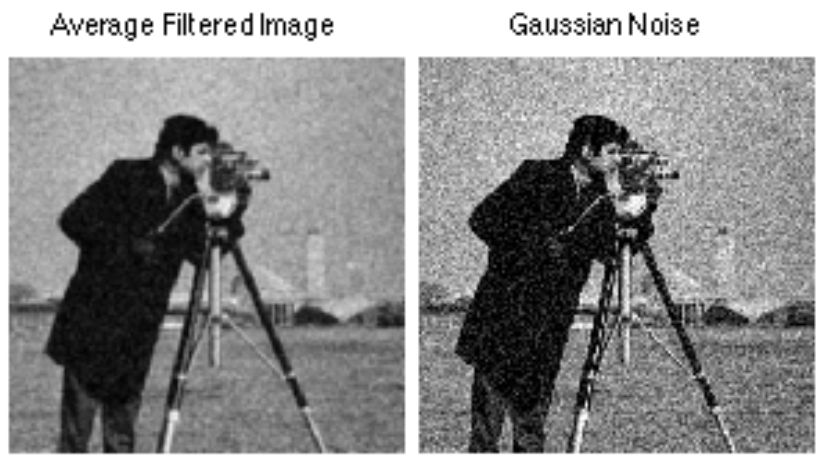
- Credit to Ray Phan for the image
- Elastic transformation
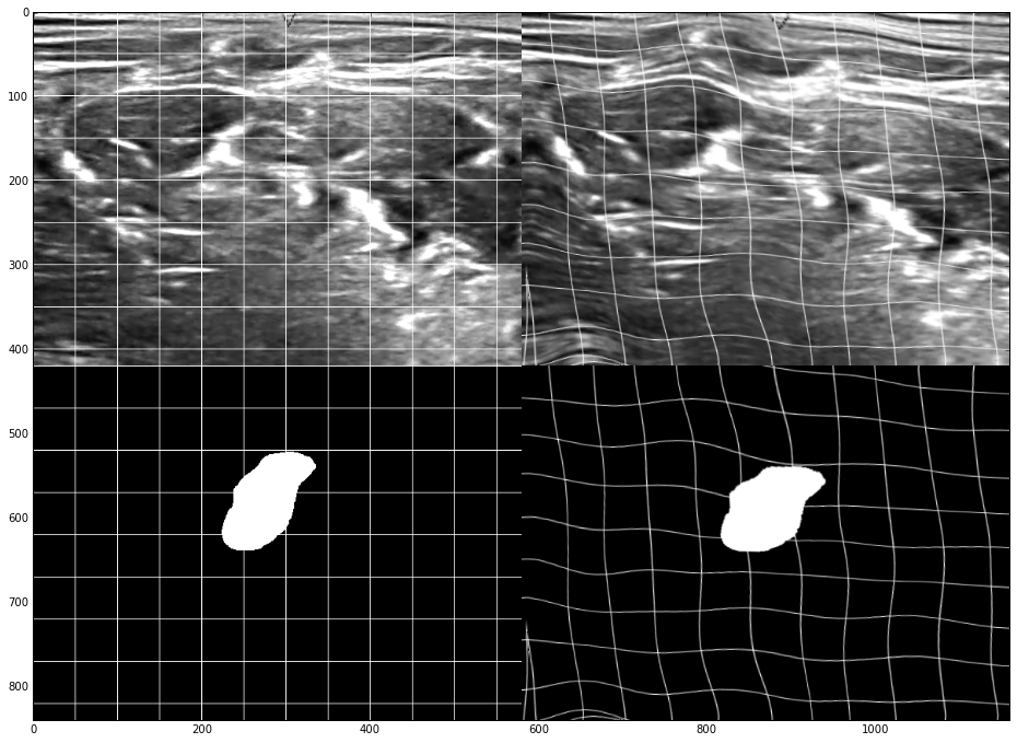
- Credit to Bruno G. do Amaral for the image
The idea is that these modified images will make the model more robust by both having additional training samples (reducing chances of underfitting) and due to having more noise and variation in the training set (reducing chances of overfitting).
For this competition, I used image rotation and shifting. Elastic deformation would’ve likely helped with performance, but I didn’t implement it due to time constraints.
Neural Network
Here’s the architecture of the neural network and a brief description of the components:
Conv(5,5) -> Conv(5,5) -> MaxPooling -> Dropout (50%) -> Conv(3,3) -> Conv(3,3) -> MaxPooling -> Dropout (50%) -> FC1024 Dropout (50%) -> FC1024 -> SoftMax
Note: Replace text with image
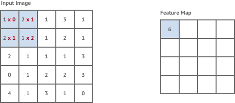
- Convolutional Layers: These layers are a little more abstract than typical fully connected layers because they incorporate spatial aspects of the input data. More specifically, they scan over the input data (the image in this case) and create filters (also referred to as kernels or feature maps) that look for specific features that the model deems important - this is a kind of automatic feature engineering by finding representation within the data automatically. For images, these filters are usually things like colors, edges, corners, textures, or even more complex shapes. Below is a high level example of a convolutional layer scanning over an image and creating filters:
-

- Credit to Microsoft for the gif
- Note: In this image we are constructing filters for multiple channels, or colors, but this project used greyscale images. A more accurate representation would be one grey layer on the top of the gif.
-
Here is a more specific view of creating the filter by multiplying pixel intensities (the numbers under the input image) by trainable weights:
- Below is an example of filters at different levels of the convolutional network that demonstrates how the learned features get more complex deeper in the network:
-
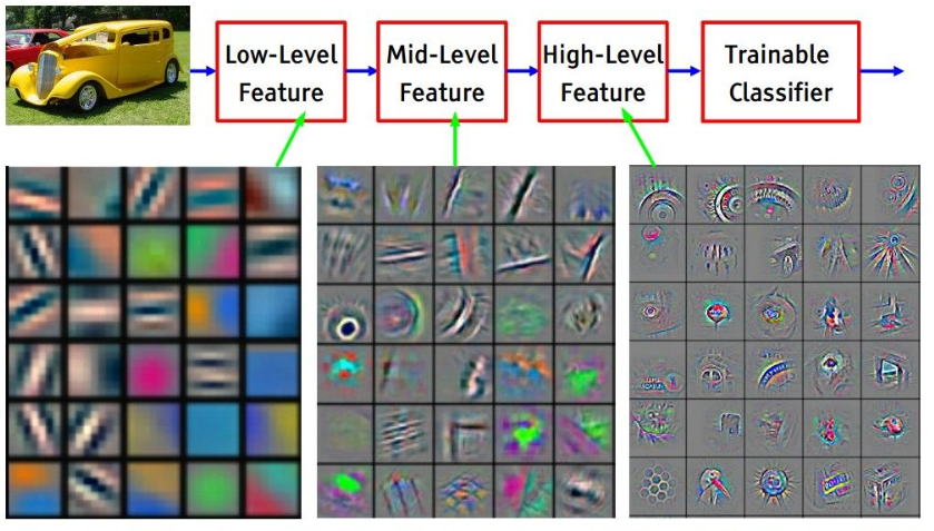
- Credit to Stanford University for the image
-
- These layers also all used batch normalization and ReLU activations
- Batch Normalization: This helps the network learn faster and obtain higher accuracy by scaling the hidden units to a comparable range. This also allows our network to be more stable due to not having large discrepancies in values. Lastly, this helps us avoid the “internal covariate shift” problem where small changes to the network are amplified further on in the network, thus causing a change in the input distribution to internal layers of the network.
- Rectified Linear Unit (ReLU) Activations: Activation functions are used in neural networks because they apply non-linear functions to the hidden layers, thus allowing the model to learn more complex functional mappings from data. Sigmoid and TanH activations were previously the most popular activation methods, but recent research has shown that ReLUs tend to outperform other activation methods. The first reason is because it can learn faster due to a reduced likelihood of having a vanishing gradient - this is where a the gradient becomes extremely small as the absolute value of x increases. The second reason is sparsity, which is a nice property that allows faster training.
-
- Max Pooling: This allows us to train the network faster by reducing the number of parameters while still retaining a large amount of information. Below is an image of 2x2 max pooling over a 4x4 filter.
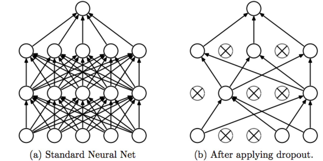
- Dropout: Dropout is a regularization technique that randomly de-activates components of a neural network at random. It seems counter-intuitive at first, but it helps the neurons become more robust by forcing them to generalize more in order to obtain good performance when other neurons are randomly being de-activated. This is also an extreme form of bagging (bootstrap aggregating) because our neural network is effectively a different one at each mini-batch due to different neurons being active.
- Fully Connected Layers: These are the traditional layers like those pictured in the dropout example above. These layers take the features learned from the convolutional layers and do the actual classification.
- Softmax: This is the final piece of our neural network where we take the outputs for a given image and scale them into probabilities (with the sum of the probabilities for all images adding up to 1) in order to generate our prediction.

The general idea of the network is that the convolutional layers learn the features (ex. the edges/corners/shapes/color intensity differences) that the fully connected layers then use to classify the images. This is one of the key differences between deep learning and traditional machine learning - performing automatic engineering by learning representations or encoding the data. A traditional machine learning model, logistic regression for example, would generally just learn the importance of the color intensity for each given pixel, but not how important the pixels are together.
Because of this automatic feature engineering, transfer learning, a method where only the fully connected layers are re-trained in order to classify specific images, is extremely popular. While this is a very simplified explanation, this is how things ilke Microsoft’s Custom Vision Service work.
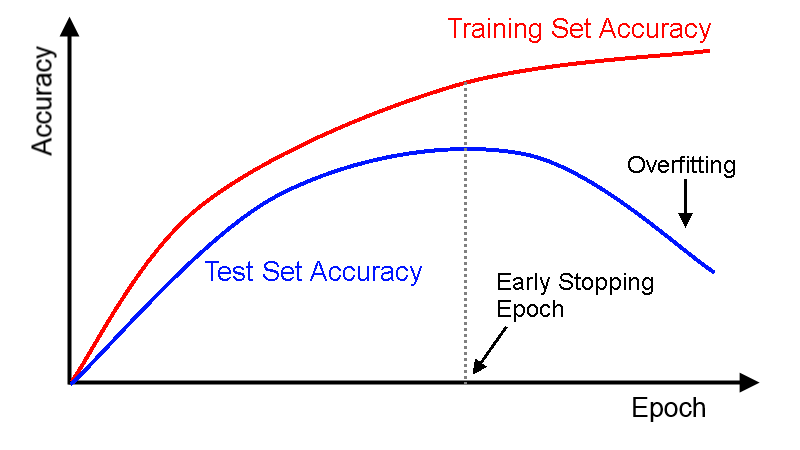
Early Stopping
One thing I wanted to mention that I didn’t add to my script that I should have was early stopping. Early stopping is a unique regularization technique that is very computationally efficient to implement. It prevents overfitting by stopping the training of our model when the validation accuracy begins to decrease relative to our training accuracy:
Credit to DL4J for the image
This is extremely efficient because it not only prevents unnecessary training that inadvertently harms the generalization, but it is more or less a self-learning parameter - we don’t have to re-train the model using different values because the optimal value is decided during training.
Final Thoughts
Overall, the competition was a great learning experience. I’ve played around with deep learning in the past, but this really forced me to learn how to correctly use different concepts to build an effective model. Here are a few other thoughts:
- TensorFlow is an extremely popular deep learning framework, but it is not nearly as easy to use as higher level libraries like Keras
- TensorFlow does have other neat tools like TensorBoard that I didn’t end up taking advantage of
- Loading saved models and generating predictions is not trivial in TensorFlow
- GPUs are essential for any kind of serious deep learning work
- CUDA and cuDNN, the toolkits required to use an NVIDIA GPU with deep learning libraries, are not as difficult as they seem to set up
- GPU memory matters - my 5 year old GPU has much less memory than GPUs today, and as a result my mini-batches had to be smaller (resulting in a slower training speed and reduced accuracy)
- fast.ai by Jeremy Howard and Rachel Thomas and Deep Learning by Yoshua Bengio, Ian Goodfellow, and Aaron Courville were fantastic learning resources
- I plan on writing a post in the future with all of the “rules of thumb” from Deep Learning after I finish reading it cover to cover - stay tuned!
Code
Here’s the unedited script used to train the winning model.
from __future__ import division, print_function, absolute_import

import sys
import os
import numpy as np
import tensorflow as tf
import pickle
from datetime import datetime
import time

print('OS: ', sys.platform)
print('Python: ', sys.version)
print('NumPy: ', np.__version__)
print('TensorFlow: ', tf.__version__)

# Checking TensorFlow processing devices
from tensorflow.python.client import device_lib
local_device_protos = device_lib.list_local_devices()
print([x for x in local_device_protos if x.device_type == 'GPU'])

# GPU memory management settings
config = tf.ConfigProto()
# config.gpu_options.allow_growth = True
config.gpu_options.per_process_gpu_memory_fraction = 0.2

# Importing the data
dir_path = os.path.dirname(os.path.realpath(__file__))
pickle_file = 'notMNIST.pickle'

with open(dir_path+'\\'+pickle_file, 'rb') as f:
    save = pickle.load(f, encoding='iso-8859-1')
    X_train = save['train_dataset']
    y_train = save['train_labels']
    X_validation = save['valid_dataset']
    y_validation = save['valid_labels']
    X_test = save['test_dataset']
    y_test = save['test_labels']
    del save  # hint to help gc free up memory
    print('\nNative data shapes:')
    print('Training set', X_train.shape, y_train.shape)
    print('Validation set', X_validation.shape, y_validation.shape)
    print('Test set', X_test.shape, y_test.shape, '\n')

image_size = 28
num_labels = 10
num_channels = 1  # grayscale

# Reformatting to unflattened images
def reformat(dataset, labels):
    dataset = dataset.reshape((-1, image_size, image_size, num_channels)).astype(np.float32)
    labels = (np.arange(num_labels) == labels[:,None]).astype(np.float32)
    return dataset, labels

X_train, y_train = reformat(X_train, y_train)
X_validation, y_validation = reformat(X_validation, y_validation)
X_test, y_test = reformat(X_test, y_test)

print('Reformatted data shapes:')
print('Training set', X_train.shape, y_train.shape)
print('Validation set', X_validation.shape, y_validation.shape)
print('Test set', X_test.shape, y_test.shape, '\n')


# Augment training data
def augment_training_data(images, labels):
    """
    Generates augmented training data by rotating and shifting images
    Creates an additional 300,000 training samples

    Takes ~1.25 minutes with an i7/16gb machine
    """
    from scipy import ndimage

    # Empty lists to fill
    expanded_images = []
    expanded_labels = []

    # Looping through samples, modifying them, and appending them to the empty lists
    j = 0   # counter
    for x, y in zip(images, labels):
        j = j + 1
        if j % 10000 == 0:
            print('Expanding data: %03d / %03d' % (j, np.size(images, 0)))

        # register original data
        expanded_images.append(x)
        expanded_labels.append(y)

        # get a value for the background
        # zero is the expected value, but median() is used to estimate background's value
        bg_value = np.median(x)  # this is regarded as background's value
        image = np.reshape(x, (-1, 28))

        for i in range(4):
            # rotate the image with random degree
            angle = np.random.randint(-15, 15, 1)
            new_img = ndimage.rotate(
                image, angle, reshape=False, cval=bg_value)

            # shift the image with random distance
            shift = np.random.randint(-2, 2, 2)
            new_img_ = ndimage.shift(new_img, shift, cval=bg_value)

            # register new training data
            expanded_images.append(np.reshape(new_img_, (28, 28, 1)))
            expanded_labels.append(y)

    return expanded_images, expanded_labels


print('Starting')
augmented = augment_training_data(X_train, y_train)
print('Completed')

# Appending to the end of the current X/y train
X_train_aug = np.append(X_train, augmented[0], axis=0)
y_train_aug = np.append(y_train, augmented[1], axis=0)

print('X_train shape:', X_train_aug.shape)
print('y_train shape:', y_train_aug.shape)
print(X_train_aug.shape[0], 'Train samples')
print(X_validation.shape[0], 'Validation samples')
print(X_test.shape[0], 'Test samples')


def accuracy(predictions, labels):
    return (100.0 * np.sum(np.argmax(predictions, 1) == np.argmax(labels, 1)) / predictions.shape[0])

# Training Parameters
learning_rate = 0.001
num_steps = y_train.shape[0] + 1  # 200,000 per epoch
batch_size = 128
epochs = 100
display_step = 250  # To print progress

# Network Parameters
num_input = 784  # Data input (image shape: 28x28)
num_classes = 10  # Total classes (10 characters)

graph = tf.Graph()

with graph.as_default():
    # Input data
    tf_X_train = tf.placeholder(tf.float32, shape=(batch_size, image_size, image_size, num_channels))
    tf_y_train = tf.placeholder(tf.float32, shape=(batch_size, num_labels))
    tf_X_validation = tf.constant(X_validation)
    tf_X_test = tf.constant(X_test)

    # Create some wrappers for simplicity
    def maxpool2d(x, k=2):
        """
        Max Pooling wrapper
        """
        return tf.nn.max_pool(x, ksize=[1, k, k, 1], strides=[1, k, k, 1], padding='SAME')

    def batch_norm(x):
        """
        Batch Normalization wrapper
        """
        return tf.contrib.layers.batch_norm(x, center=True, scale=True, fused=True,)

    def conv2d(data, outputs=32, kernel_size=(5, 5), stride=1, regularization=0.00005):
        """
        Conv2D wrapper, with bias and relu activation
        """
        layer = tf.contrib.layers.conv2d(inputs=data,
                                         num_outputs=outputs,
                                         kernel_size=kernel_size,
                                         stride=stride,
                                         padding='SAME',
                                         weights_regularizer=tf.contrib.layers.l2_regularizer(scale=regularization),
                                         biases_regularizer=tf.contrib.layers.l2_regularizer(scale=regularization))
        return layer

    # Conv(5,5) -> Conv(5,5) -> MaxPooling -> Conv(3,3) -> Conv(3,3) -> MaxPooling -> FC1024 -> FC1024 -> SoftMax
    def model(x):
        # Conv(5, 5)
        conv1 = conv2d(x)
        bnorm1 = batch_norm(conv1)

        # Conv(5, 5) -> Max Pooling
        conv2 = conv2d(bnorm1, outputs=64)
        bnorm2 = batch_norm(conv2)
        pool1 = maxpool2d(bnorm2, k=2)  # 14x14
        drop1 = tf.nn.dropout(pool1, keep_prob=0.5)

        # Conv(3, 3)
        conv3 = conv2d(drop1, outputs=64, kernel_size=(3, 3))
        bnorm3 = batch_norm(conv3)

        # Conv(3, 3) -> Max Pooling
        conv4 = conv2d(bnorm3, outputs=64, kernel_size=(3, 3))
        bnorm4 = batch_norm(conv4)
        pool2 = maxpool2d(bnorm4, k=2)  # 7x7
        drop2 = tf.nn.dropout(pool2, keep_prob=0.5)

        # FC1024
        # Reshape conv2 output to fit fully connected layer input
        flatten = tf.contrib.layers.flatten(drop2)
        fc1 = tf.contrib.layers.fully_connected(
            flatten,
            1024,
            weights_regularizer=tf.contrib.layers.l2_regularizer(scale=0.00005),
            biases_regularizer=tf.contrib.layers.l2_regularizer(scale=0.00005),
        )
        drop3 = tf.nn.dropout(fc1, keep_prob=0.5)

        # FC1024
        fc2 = tf.contrib.layers.fully_connected(
            fc1,
            1024,
            weights_regularizer=tf.contrib.layers.l2_regularizer(scale=0.00005),
            biases_regularizer=tf.contrib.layers.l2_regularizer(scale=0.00005),
        )

        # Output, class prediction
        out = tf.contrib.layers.fully_connected(
            fc2,
            10,
            activation_fn=None,
            weights_regularizer=tf.contrib.layers.l2_regularizer(scale=0.00005),
            biases_regularizer=tf.contrib.layers.l2_regularizer(scale=0.00005),
        )
        return out

    # Construct model
    logits = model(tf_X_train)

    prediction = tf.nn.softmax(logits)

    # Define loss and optimizer
    loss = tf.reduce_mean(tf.nn.softmax_cross_entropy_with_logits(labels=tf_y_train, logits=logits))
    optimizer = tf.train.GradientDescentOptimizer(0.05).minimize(loss)


# Initialize the variables (i.e. assign their default value)
init = tf.global_variables_initializer()

# Start training
with tf.Session(config=config, graph=graph) as session:
    tf.global_variables_initializer().run()
    print('Initialized')

    # For tracking execution time and progress
    start_time = time.time()
    total_steps = 0

    for epoch in range(1, epochs+1):
        print('Beginning Epoch {0} -'.format(epoch))

        def next_batch(num, data, labels):
            """
            Return a total of `num` random samples and labels.
            Mimicks the mnist.train.next_batch() function
            """
            idx = np.arange(0 , len(data))
            np.random.shuffle(idx)
            idx = idx[:num]
            data_shuffle = [data[i] for i in idx]
            labels_shuffle = [labels[i] for i in idx]

            return np.asarray(data_shuffle), np.asarray(labels_shuffle)


        for step in range(num_steps):
            batch_data, batch_labels = next_batch(batch_size, X_train_aug, y_train_aug)

            feed_dict = {tf_X_train: batch_data, tf_y_train: batch_labels}
            _, l, predictions = session.run([optimizer, loss, train_prediction], feed_dict=feed_dict)

            if (step % 250 == 0) or (step == num_steps):
                # Calculating percentage of completion
                total_steps += step
                pct_epoch = (step / float(num_steps)) * 100
                pct_total = (total_steps / float(num_steps * (epochs+1))) * 100  # Fix this line

                # Printing progress
                print('Epoch %d Step %d (%.2f%% epoch, %.2f%% total)' % (epoch, step, pct_epoch, pct_total))
                print('------------------------------------')
                print('Minibatch loss: %f' % l)
                print('Minibatch accuracy: %.1f%%' % accuracy(predictions, batch_labels))
                print(datetime.now())
                print('Total execution time: %.2f minutes' % ((time.time() - start_time)/60.))
                print()

        # Save the model every 5th epoch
        if epoch % 5 == 0:
            # Saver object - saves model as 'tfTestModel_20epochs_Y-M-D_H-M-S'
            saver = tf.train.Saver()
            current_time = datetime.now().strftime("%Y-%m-%d_%H-%M-%S")
            saver.save(session, dir_path+'\\models\\'+'tfTestModel'+'_'+str(epoch)+'epochs_'+str(current_time))
            print('Saving model at current stage')

    # Saver object - saves model as 'tfTestModel_20epochs_Y-M-D_H-M-S'
    saver = tf.train.Saver()
    current_time = datetime.now().strftime("%Y-%m-%d_%H-%M-%S")
    saver.save(session, dir_path+'\\models\\'+'tfTestModel'+'_'+str(epoch)+'epochs_'+str(current_time))
print('Complete')