
Restaurant Recommender
Introduction
In this project, I extracted restaurant ratings and reviews from Foursquare and used distance (one of the main ideas behind recommender systems) to generate recommendations for restaurants in one city that have similar reviews to restaurants in another city. This post is the abridged version, but check out my github post for all of the code if you are curious or want to use it.
Motivation
I grew up in Austin, Texas, and moved to Minneapolis, Minnesota a few years ago. My wife and I are people who love food, and loved the food culture in Austin. After our move, we wanted to find new restaurants to replace our favorites from back home. However, most decently rated places in Minneapolis we went to just didn’t quite live up to our Austin expectations. These restaurants usually came at the recommendations of locals, acquaintances, or from Google ratings, but the food was often bland and overpriced. It took us one deep dive into the actual reviews to figure it out.
In order to better illustrate our problem, below are recent reviews from three restaurants that left us disappointed. On the left is a typical American restaurant, the middle is a Vietnamese restaurant, and the right is a pizza shop:

I highlighted the main points to stand out against the small font. Service, atmosphere, and apparently eggrolls were the most common and unifying factors. You see very little discussion on the quality of the actual food, and you can even see an instance where a reviewer rates the pizza place as 5/5 even after saying that it is expensive. I began to notice a disconnect in how I evaluate restaurants versus how the people of Minneapolis evaluate restaurants. If you have previously worked with recommender systems, you already know where I’m going with this. If not, here is a primer:
Recommender Systems Overview
Before getting into the overview of recommender systems, I wanted to point out that I won’t actually be building a legitimate recommender system in this notebook. There are some great packages for doing so, but I’m going to stick with one of the main ideas behind recommender systems. This is for two reasons:
1) Classes have started back up, and my available free time for side projects like this one is almost non-existant.
2) My gastronomic adventures don’t need the added benefits that a recommender system provides over what I’ll be doing.
Let’s get back into it.
In the world of recommender systems, there are three broad types:
- Collaborative Filtering (user-user): This is the most prevalent type of recommender systems that uses “wisdom of the crowd” for popularity among peers. This option is particularly popular because you don’t need to know a lot about the item itself, you only need the ratings submitted by reviewers. The two primary restrictions are that it makes the assumption that peoples’ tastes do not change over time, and new items run into the “cold start problem”. This is when either a new item has not yet received any ratings and fails to appear on recommendation lists, or a new user has not reviewed anything so we don’t know what their tastes are.
- E.x.: People who like item X also like item Y
- This is how Spotify selects songs for your recommended play list. Specifically, it will take songs from other play lists that contain songs you recently liked.
- E.x.: People who like item X also like item Y
- Content-Based (item-item): This method recommends items based off of their similarity to other items. This requires reliable information about the items themselves, which makes it difficult to implement in a lot of cases. Additionally, recommendations generated from this will option likely not deviate very far from the item being compared to, but there are tricks available to account for this.
- E.x.: Item X is similar to item Y
- This is how Pandora selects songs for your stations. Specifically, it assigns each song a list of characteristics (assigned through the Music Genome Project), and selects songs with similar characteristics as those that you liked.
- E.x.: Item X is similar to item Y
- Hybrid: You probably guessed it - this is a combination of the above two types. The idea here is use what you have if you have it. Here are a few designs related to this that are worth looking into.
Those are the three main types, but there is one additional type that you may find if you are diving a little deeper into the subject material:
- Knowledge-Based: This is is the most rare type mainly because it requires explicit domain knowledge. It is often used for products that have a low number of available ratings, such as high luxury goods like hypercars. We won’t delve any further into this type, but I recommend reading more about it if you’re interested in the concept.
Methodology
Let’s return to our problem. The previous way of selecting restaurants at the recommendation of locals and acquaintances (collaborative filtering) wasn’t always successful, so we are going to use the idea behind content-based recommender systems to evaluate our options. However, we don’t have a lot of content about the restaurants available, so we are going to primarily use the reviews people left for them. More specifically, we are going to determine similarity between restaurants based off of the similarity of the reviews that people have written for them.
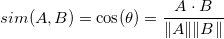
We’re going to use cosine similarity since it’s generally accepted as producing better results in item-to-item filtering:
Before calculating this, we need to perform a couple of pre-processing steps on our reviews in order to make the data usable for our cosine similarity calculation. These will be common NLP (natural language processing) techniques that you should be familiar with if you have worked with text before. These are the steps I took, but I am open to feedback and improvement if you have recommendations on other methods that may yield better results.
1) Normalizing: This step converts our words into lower case so that when we map to our feature space, we don’t end up with redundant features for the same words.
Before:
After:
2) Tokenizing: This step breaks up a sentence into individual words, essentially turning our reviews into bags of words, which makes it easier to perform other operations. Though we are going to perform many other preprocessing operations, this is more or less the beginning of mapping our reviews into the feature space.
Before:
After:
3) Removing Stopwords and Punctuation: This step removes unnecessary words and punctuation often used in language that computers don’t need such as as, the, and, and of.
Before:
After:
4) Lemmatizing (Stemming): Lemmatizing (which is very similar to stemming) removes variations at the end of a word to revert words to their root word.
Before:
After:
5) Term Frequency-Inverse Document Frequency (TF-IDF): This technique determines how important a word is to a document (which is a review in this case) within a corpus (the collection documents, or all reviews). This doesn’t necessarily help establish context within our reviews themselves (for example, ‘this Pad Kee Mao is bad ass’ is technically a good thing, which wouldn’t be accounted for unless we did n-grams (which will give my laptop a much more difficult time)), but it does help with establishing the importance of the word.

On a side note, sarcasm, slang, misspellings, emoticons, and context are common problems in NLP, but we will be ignoring these due to time limitations.
Assumptions
It’s always important to state your assumptions in any analysis because a violation of them will often impact the reliability of the results. My assumptions in this case are as follows:
- The reviews are indicative of the characteristics of the restaurant.
- The language used in the reviews does not directly impact the rating a user gives.
- E.g. Reviews contain a description of their experience, but ratings are the result of the user applying weights to specific things they value.
- Ex. “The food was great, but the service was terrible.” would be a 2/10 for one user, but a 7/10 for users like myself.
- E.g. Reviews contain a description of their experience, but ratings are the result of the user applying weights to specific things they value.
- The restaurants did not undergo significant changes in the time frame for the reviews being pulled.
- Sarcasm, slang, misspellings, and other common NLP problems will not have a significant impact on our results.
Restaurant Recommender
If you’re still with us after all of that, let’s get started!
We’ll be using standard libraries for this project (pandas, nltk, and scikit-learn), but one additional thing we need for this project are credentials to access the Foursquare API. I’m not keen on sharing mine, but you can get your own by signing up.
The Data
Foursquare works similarly to Yelp where users will review restaurants. They can either leave a rating (1-10), or write a review for the restaurant. The reviews are what we’re interested in here since I established above that the rating has less meaning due to the way people rate restaurants differently between the two cities.
The documentation was fortunately fairly robust, and you can read about the specific API calls I used in my github code. I had to perform a few calls in order to get all of the data I needed, but the end result is a data frame with one row for each of the ~1,100 restaurants and a column (comments) that contains all of the reviews:
| id | name | category | shortCategory | checkinsCount | city | state | location | commentsCount | usersCount | priceTier | numRatings | rating | comments | |
|---|---|---|---|---|---|---|---|---|---|---|---|---|---|---|
| 0 | 4e17b348b0fb8567c665ddaf | Souper Salad | Salad Place | Salad | 1769 | Austin | TX | Austin, TX | 17 | 683 | 1.0 | 41.0 | 6.9 | {Healthy fresh salad plus baked potatoes, sele... |
| 1 | 4aceefb7f964a52013d220e3 | Aster's Ethiopian Restaurant | Ethiopian Restaurant | Ethiopian | 1463 | Austin | TX | Austin, TX | 34 | 1018 | 2.0 | 93.0 | 8.0 | {The lunch buffet is wonderful; everything is ... |
| 2 | 4b591015f964a520c17a28e3 | Taste Of Ethiopia | Ethiopian Restaurant | Ethiopian | 1047 | Pflugerville | TX | Austin, TX | 31 | 672 | 2.0 | 88.0 | 8.3 | {Wonderful! Spicy lovers: Kitfo, was awesome! ... |
| 3 | 4ead97ba4690615f26a8adfe | Wasota African Cuisine | African Restaurant | African | 195 | Austin | TX | Austin, TX | 12 | 140 | 2.0 | 10.0 | 6.2 | {Obsessed with this place. One little nugget (... |
| 4 | 4c7efeba2042b1f76cd1c1ad | Cazamance | African Restaurant | African | 500 | Austin | TX | Austin, TX | 11 | 435 | 1.0 | 15.0 | 8.0 | {West African fusion reigns at this darling tr... |
I excluded fast food restaurants and chains from my API call since I’m not interested in them, but a few were included due to having a different category assigned to them. For example, most of the restaurants under the “coffee” category are Starbucks.
Let’s look at a few charts for exploratory analysis to get a better idea of our data, starting with the number of reviews per restaurant:
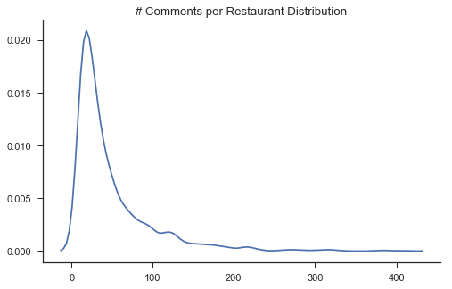
One thing to note is that I’m currently limited to 30 comments per restaurant ID since I’m using a free developer key, so this will impact the quality of the analysis to a degree.
Next, let’s look at the number of restaurants per city:
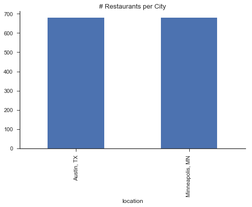
These appear to be even, so let’s look at the breakdown of restaurant categories between the two cities:
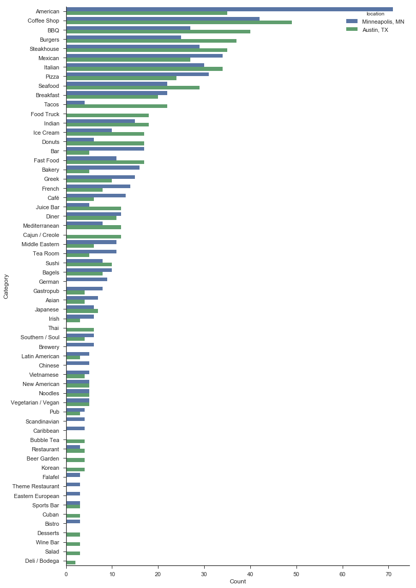
To summarize this chart:
Austin:
- Significantly more BBQ, tacos, food trucks, donuts, juice bars, and Cajun restaurants (but I could have told you this)
- Seemingly more diversity in the smaller categories
Minneapolis:
- American is king
- Significantly more bars, bakeries, middle eastern, cafés, tea rooms, German, and breweries
Lastly, here’s an example of the comments for one random restaurant to give a better idea of the text that we’re dealing with:
Data Processing
When working with language, we have to process the text into something that a computer can handle more easily. Our end result will be a large number of numerical features for each restaurant that we can use to calculate the cosine similarity.
The steps here are:
- Normalizing
- Tokenizing
- Removing stopwords
- Lemmatizing (Stemming)
- Term Frequency-Inverse Document Frequency (TF-IDF)
I’ll explain a little more on what these are and why we are doing them below in case you aren’t familiar with them.
1) Normalizing
This section uses regex scripts that makes cases every word lower cased, removes punctuation, and removes digits.
For example:
Before:
After:
The benefit in this is that it vastly reduces our feature space. Our pre-processed example would have created an additional two features if someone else used the words ‘central’ and ‘texas’ in their review.
%%time

# Converting all words to lower case and removing punctuation
df['comments'] = [re.sub(r'\d+\S*', '',
                  row.lower().replace('.', ' ').replace('_', '').replace('/', ''))
                  for row in df['comments']]

df['comments'] = [re.sub(r'(?:^| )\w(?:$| )', '', row)
                  for row in df['comments']]

# Removing numbers
df['comments'] = [re.sub(r'\d+', '', row) for row in df['comments']]
Wall time: 971 ms
2) Tokenizing
Tokenizing a sentence is a way to map our words into a feature space. This is achieved by treating every word as an individual object.
For example:
Before:
After:
%%time

# Tokenizing comments and putting them into a new column
tokenizer = nltk.tokenize.RegexpTokenizer(r'\w+')  # by blank space
df['tokens'] = df['comments'].apply(tokenizer.tokenize)
Wall time: 718ms
3) Removing Stopwords & Punctuation
Stopwords are unnecessary words like as, the, and, and of that aren’t very useful for our purposes. Since they don’t have any intrinsic value, removing them reduces our feature space which will speed up our computations.
For example:
Before:
After:
This does take a bit longer to run at ~5 minutes
%%time

filtered_words = []
for row in df['tokens']:
    filtered_words.append([
        word.lower() for word in row
        if word.lower() not in nltk.corpus.stopwords.words('english')
    ])

df['tokens'] = filtered_words
Wall time: 4min 59s
4) Lemmatizing (Stemming)
Stemming removes variations at the end of a word to revert words to their root in order to reduce our overall feature space (e.x. running –> run). This has the possibility to adversely impact our performance when the root word is different (e.x. university –> universe), but the net positives typically outweigh the net negatives.
For example:
Before:
After:
One very important thing to note here is that we’re actually doing something called Lemmatization, which is similar to stemming, but is a little different. Both seek to reduce inflectional forms and sometimes derivationally related forms of a word to a common base form, but they go about it in different ways. In order to illustrate the difference, here’s a dictionary entry:

Lemmatization seeks to get the lemma, or the base dictionary form of the word. In our example above, that would be “graduate”. It does this by using vocabulary and a morphological analysis of the words, rather than just chopping off the variations (the “verb forms” in the example above) like a traditional stemmer would.
The advantage of lemmatization here is that we don’t run into issues like our other example of university –> universe that can happen in conventional stemmers. It is also relatively quick on this data set!
The disadvantage is that it is not able to infer if the word is a noun/verb/adjective/etc., so we have to specify which type it is. Since we’re looking at, well, everything, we’re going to lemmatize for nouns, verbs, and adjectives.
Here is an excerpt from the Stanford book Introduction to Information Retrieval if you wanted to read more stemming and lemmatization.
%%time

# Setting the Lemmatization object
lmtzr = nltk.stem.wordnet.WordNetLemmatizer()

# Looping through the words and appending the lemmatized version to a list
stemmed_words = []
for row in df['tokens']:
    stemmed_words.append([
        # Verbs
        lmtzr.lemmatize(
            # Adjectives
            lmtzr.lemmatize(
                # Nouns
                lmtzr.lemmatize(word.lower()), 'a'), 'v')
        for word in row
        if word.lower() not in nltk.corpus.stopwords.words('english')])

# Adding the list as a column in the data frame
df['tokens'] = stemmed_words
Wall time: 4min 52s
Let’s take a look at how many unique words we now have and a few of the examples:
# Appends all words to a list in order to find the unique words
allWords = []
for row in stemmed_words:
    for word in row:
        allWords.append(str(word))

uniqueWords = np.unique(allWords)

print('Number of unique words:', len(uniqueWords), '\n')
print('Previewing sample of unique words:\n', uniqueWords[1234:1244])
Number of unique words: 36592

Previewing sample of unique words:
 ['andhitachino' 'andhome' 'andhomemade' 'andhopping' 'andhot' 'andhouse'
 'andhuge' 'andiamo' 'andimmediatly' 'andis']
We can see a few of the challenges from slang or typos that I mentioned in the beginning. These will pose problems for what we’re doing, but we’ll just have to assume that the vast majority of words are spelled correctly.
Before doing the TF-IDF transformation, we need to make sure that we have spaces in between each word in the comments:
stemmed_sentences = []

# Spacing out the words in the reviews for each restaurant
for row in df['tokens']:
    stemmed_string = ''
    for word in row:
        stemmed_string = stemmed_string + ' ' + word
    stemmed_sentences.append(stemmed_string)

df['tokens'] = stemmed_sentences
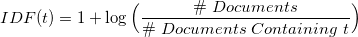
5) Term Frequency-Inverse Document Frequency (TF-IDF)
This determines how important a word is to a document (which is a review in this case) within a corpus (the collection documents). It is a number resulting from the following formula:
Scikit-learn has an excellent function that is able to transform our processed text into a TF-IDF matrix very quickly. We’ll convert it back to a data frame, and join it to our original data frame by the indexes.
%%time

# Creating the sklearn object
tfidf = sktext.TfidfVectorizer(smooth_idf=False)

# Transforming our 'tokens' column into a TF-IDF matrix and then a data frame
tfidf_df = pd.DataFrame(tfidf.fit_transform(df['tokens']).toarray(),
                        columns=tfidf.get_feature_names())
Wall time: 1.47 s
print(tfidf_df.shape)
tfidf_df.head()
(1335, 36571)
| aa | aaa | aaaaaaa | aaaaaaamazing | aaaaaamaaaaaaazing | aaaaalll | aaaaand | aaaammaazzing | aaallllllll | aaarrrggghhh | ... | zucca | zucchini | zuccini | zuccotto | zuchini | zuke | zuppa | zur | zushi | zzzzzzzzzzzzoops | |
|---|---|---|---|---|---|---|---|---|---|---|---|---|---|---|---|---|---|---|---|---|---|
| 0 | 0.0 | 0.0 | 0.0 | 0.0 | 0.0 | 0.0 | 0.0 | 0.0 | 0.0 | 0.0 | ... | 0.0 | 0.0 | 0.0 | 0.0 | 0.0 | 0.0 | 0.0 | 0.0 | 0.0 | 0.0 |
| 1 | 0.0 | 0.0 | 0.0 | 0.0 | 0.0 | 0.0 | 0.0 | 0.0 | 0.0 | 0.0 | ... | 0.0 | 0.0 | 0.0 | 0.0 | 0.0 | 0.0 | 0.0 | 0.0 | 0.0 | 0.0 |
| 2 | 0.0 | 0.0 | 0.0 | 0.0 | 0.0 | 0.0 | 0.0 | 0.0 | 0.0 | 0.0 | ... | 0.0 | 0.0 | 0.0 | 0.0 | 0.0 | 0.0 | 0.0 | 0.0 | 0.0 | 0.0 |
| 3 | 0.0 | 0.0 | 0.0 | 0.0 | 0.0 | 0.0 | 0.0 | 0.0 | 0.0 | 0.0 | ... | 0.0 | 0.0 | 0.0 | 0.0 | 0.0 | 0.0 | 0.0 | 0.0 | 0.0 | 0.0 |
| 4 | 0.0 | 0.0 | 0.0 | 0.0 | 0.0 | 0.0 | 0.0 | 0.0 | 0.0 | 0.0 | ... | 0.0 | 0.0 | 0.0 | 0.0 | 0.0 | 0.0 | 0.0 | 0.0 | 0.0 | 0.0 |
5 rows × 36571 columns
Since we transformed all of the words, we have a sparse matrix. We don’t care about things like typos or words specific to one particular restaurant, so we’re going to remove columns that don’t have a lot of contents.
# Removing sparse columns
tfidf_df = tfidf_df[tfidf_df.columns[tfidf_df.sum() > 2.5]]

# Removing any remaining digits
tfidf_df = tfidf_df.filter(regex=r'^((?!\d).)*$')

print(tfidf_df.shape)
tfidf_df.head()
(1335, 976)
| absolute | absolutely | across | actually | add | afternoon | ahead | ahi | al | ale | ... | wow | wrap | wrong | www | year | yes | yet | york | yum | yummy | |
|---|---|---|---|---|---|---|---|---|---|---|---|---|---|---|---|---|---|---|---|---|---|
| 0 | 0.0 | 0.000000 | 0.0 | 0.000000 | 0.0 | 0.0 | 0.0 | 0.0 | 0.0 | 0.0 | ... | 0.0000 | 0.000000 | 0.000000 | 0.074605 | 0.0 | 0.0 | 0.000000 | 0.000000 | 0.000000 | 0.000000 |
| 1 | 0.0 | 0.000000 | 0.0 | 0.034778 | 0.0 | 0.0 | 0.0 | 0.0 | 0.0 | 0.0 | ... | 0.0000 | 0.000000 | 0.024101 | 0.000000 | 0.0 | 0.0 | 0.000000 | 0.000000 | 0.023301 | 0.023143 |
| 2 | 0.0 | 0.031268 | 0.0 | 0.000000 | 0.0 | 0.0 | 0.0 | 0.0 | 0.0 | 0.0 | ... | 0.0376 | 0.000000 | 0.026175 | 0.000000 | 0.0 | 0.0 | 0.000000 | 0.000000 | 0.000000 | 0.025135 |
| 3 | 0.0 | 0.000000 | 0.0 | 0.000000 | 0.0 | 0.0 | 0.0 | 0.0 | 0.0 | 0.0 | ... | 0.0000 | 0.000000 | 0.000000 | 0.000000 | 0.0 | 0.0 | 0.000000 | 0.000000 | 0.000000 | 0.000000 |
| 4 | 0.0 | 0.000000 | 0.0 | 0.000000 | 0.0 | 0.0 | 0.0 | 0.0 | 0.0 | 0.0 | ... | 0.0000 | 0.060402 | 0.000000 | 0.000000 | 0.0 | 0.0 | 0.065236 | 0.085197 | 0.000000 | 0.000000 |
5 rows × 976 columns
This drastically reduced the dimensions of our data set, and we now have something usable to calculate similarity.
# Storing the original data frame before the merge in case of changes
df_orig = df.copy()

# Renaming columns that conflict with column names in tfidfCore
df.rename(columns={'name': 'Name',
                   'city': 'City',
                   'location': 'Location'}, inplace=True)

# Merging the data frames by index
df = pd.merge(df, tfidf_df, how='inner', left_index=True, right_index=True)

df.head()
| id | Name | category | shortCategory | checkinsCount | City | state | Location | commentsCount | usersCount | ... | wow | wrap | wrong | www | year | yes | yet | york | yum | yummy | |
|---|---|---|---|---|---|---|---|---|---|---|---|---|---|---|---|---|---|---|---|---|---|
| 0 | 4e17b348b0fb8567c665ddaf | Souper Salad | Salad Place | Salad | 1769 | Austin | TX | Austin, TX | 17 | 683 | ... | 0.0000 | 0.000000 | 0.000000 | 0.074605 | 0.0 | 0.0 | 0.000000 | 0.000000 | 0.000000 | 0.000000 |
| 1 | 4aceefb7f964a52013d220e3 | Aster's Ethiopian Restaurant | Ethiopian Restaurant | Ethiopian | 1463 | Austin | TX | Austin, TX | 34 | 1018 | ... | 0.0000 | 0.000000 | 0.024101 | 0.000000 | 0.0 | 0.0 | 0.000000 | 0.000000 | 0.023301 | 0.023143 |
| 2 | 4b591015f964a520c17a28e3 | Taste Of Ethiopia | Ethiopian Restaurant | Ethiopian | 1047 | Pflugerville | TX | Austin, TX | 31 | 672 | ... | 0.0376 | 0.000000 | 0.026175 | 0.000000 | 0.0 | 0.0 | 0.000000 | 0.000000 | 0.000000 | 0.025135 |
| 3 | 4ead97ba4690615f26a8adfe | Wasota African Cuisine | African Restaurant | African | 195 | Austin | TX | Austin, TX | 12 | 140 | ... | 0.0000 | 0.000000 | 0.000000 | 0.000000 | 0.0 | 0.0 | 0.000000 | 0.000000 | 0.000000 | 0.000000 |
| 4 | 4c7efeba2042b1f76cd1c1ad | Cazamance | African Restaurant | African | 500 | Austin | TX | Austin, TX | 11 | 435 | ... | 0.0000 | 0.060402 | 0.000000 | 0.000000 | 0.0 | 0.0 | 0.065236 | 0.085197 | 0.000000 | 0.000000 |
5 rows × 991 columns
Lastly, we’re going to add additional features for the category. This just puts a heavier weight on those with the same type, so for example a Mexican restaurant will be more likely to have Mexican restaurants show up as most similar instead of Brazilian restaurants.
# Creates dummy variables out of the restaurant category
df = pd.concat([df, pd.get_dummies(df['shortCategory'])], axis=1)

df.head()
| id | Name | category | shortCategory | checkinsCount | City | state | Location | commentsCount | usersCount | ... | Tapas | Tea Room | Tex-Mex | Thai | Theme Restaurant | Turkish | Vegetarian / Vegan | Vietnamese | Wine Bar | Yogurt | |
|---|---|---|---|---|---|---|---|---|---|---|---|---|---|---|---|---|---|---|---|---|---|
| 0 | 4e17b348b0fb8567c665ddaf | Souper Salad | Salad Place | Salad | 1769 | Austin | TX | Austin, TX | 17 | 683 | ... | 0 | 0 | 0 | 0 | 0 | 0 | 0 | 0 | 0 | 0 |
| 1 | 4aceefb7f964a52013d220e3 | Aster's Ethiopian Restaurant | Ethiopian Restaurant | Ethiopian | 1463 | Austin | TX | Austin, TX | 34 | 1018 | ... | 0 | 0 | 0 | 0 | 0 | 0 | 0 | 0 | 0 | 0 |
| 2 | 4b591015f964a520c17a28e3 | Taste Of Ethiopia | Ethiopian Restaurant | Ethiopian | 1047 | Pflugerville | TX | Austin, TX | 31 | 672 | ... | 0 | 0 | 0 | 0 | 0 | 0 | 0 | 0 | 0 | 0 |
| 3 | 4ead97ba4690615f26a8adfe | Wasota African Cuisine | African Restaurant | African | 195 | Austin | TX | Austin, TX | 12 | 140 | ... | 0 | 0 | 0 | 0 | 0 | 0 | 0 | 0 | 0 | 0 |
| 4 | 4c7efeba2042b1f76cd1c1ad | Cazamance | African Restaurant | African | 500 | Austin | TX | Austin, TX | 11 | 435 | ... | 0 | 0 | 0 | 0 | 0 | 0 | 0 | 0 | 0 | 0 |
5 rows × 1090 columns
Because we introduced an additional type of feature, we’ll have to check it’s weight in comparison to the TF-IDF features:
# Summary stats of TF-IDF
print('Max:', np.max(tfidf_df.max()), '\n',
      'Mean:', np.mean(tfidf_df.mean()), '\n',
      'Standard Deviation:', np.std(tfidf_df.std()))
Max: 0.889350911658
 Mean: 0.005518928565159508
 Standard Deviation: 0.010229821082730768
The dummy variables for the restaurant type are quite a bit higher than the average word, but I’m comfortable with this since I think it has a benefit.
“Recommender System”
As a reminder, we are not using a conventional recommender system. Instead, we are using recommender system theory by calculating the cosine distance between comments in order to find restaurants with the most similar comments.
Loading in personal ratings
In order to recommend restaurants with this approach, we have to identify the restaurants to which we want to find the most similarities. I took the data frame and assigned my own ratings to some of my favorites.
# Loading in self-ratings for restaurants in the data set
selfRatings = pd.read_csv('selfRatings.csv', usecols=[0, 4])
selfRatings.head()
| id | selfRating | |
|---|---|---|
| 0 | 43c968a2f964a5209c2d1fe3 | 10.0 |
| 1 | 574481f8498e2cd16a0911a6 | NaN |
| 2 | 4cb5e045e262b60c46cb6ae0 | 9.0 |
| 3 | 49be75ccf964a520ad541fe3 | 9.0 |
| 4 | 4d8d295fc1b1721e798b1246 | NaN |
# Merging into df to add the column 'selfRating'
df = pd.merge(df, selfRatings)
Additional features & min-max scaling
We’re going to include a few additional features from the original data set to capture information that the comments may not have. Specifically:
- Popularity: checkinsCount, commentsCount, usersCount, numRatings
- Price: priceTier
We’re also going to scale these down so they don’t carry a huge advantage over everything else. I’m going to scale the popularity attributes to be between 0 and 0.5, and the price attribute to be between 0 and 1. I’ll do this by first min-max scaling everything (to put it between 0 and 1), and then dividing the popularity features in half.
# Removing everything that won't be used in the similarity calculation
df_item = df.drop(['id', 'category', 'Name', 'shortCategory', 'City', 'tokens',
                   'comments', 'state', 'Location', 'selfRating', 'rating'],
                  axis=1)

# Copying into a separate data frame to be normalized
df_item_norm = df_item.copy()

columns_to_scale = ['checkinsCount', 'commentsCount',
                    'usersCount', 'priceTier', 'numRatings']

# Split
df_item_split = df_item[columns_to_scale]
df_item_norm.drop(columns_to_scale, axis=1, inplace=True)

# Apply
df_item_split = pd.DataFrame(MinMaxScaler().fit_transform(df_item_split),
                             columns=df_item_split.columns)
df_item_split_half = df_item_split.drop('priceTier', axis=1)
df_item_split_half = df_item_split_half / 2
df_item_split_half['priceTier'] = df_item_split['priceTier']

# Combine
df_item_norm = df_item_norm.merge(df_item_split,
                                  left_index=True, right_index=True)

df_item_norm.head()
| absolute | absolutely | across | actually | add | afternoon | ahead | ahi | al | ale | ... | Turkish | Vegetarian / Vegan | Vietnamese | Wine Bar | Yogurt | checkinsCount | commentsCount | usersCount | priceTier | numRatings | |
|---|---|---|---|---|---|---|---|---|---|---|---|---|---|---|---|---|---|---|---|---|---|
| 0 | 0.0 | 0.000000 | 0.0 | 0.000000 | 0.0 | 0.0 | 0.0 | 0.0 | 0.0 | 0.0 | ... | 0 | 0 | 0 | 0 | 0 | 0.030682 | 0.017544 | 0.020429 | 0.000000 | 0.017494 |
| 1 | 0.0 | 0.000000 | 0.0 | 0.034778 | 0.0 | 0.0 | 0.0 | 0.0 | 0.0 | 0.0 | ... | 0 | 0 | 0 | 0 | 0 | 0.024844 | 0.060150 | 0.031648 | 0.333333 | 0.046840 |
| 2 | 0.0 | 0.031268 | 0.0 | 0.000000 | 0.0 | 0.0 | 0.0 | 0.0 | 0.0 | 0.0 | ... | 0 | 0 | 0 | 0 | 0 | 0.016906 | 0.052632 | 0.020060 | 0.333333 | 0.044018 |
| 3 | 0.0 | 0.000000 | 0.0 | 0.000000 | 0.0 | 0.0 | 0.0 | 0.0 | 0.0 | 0.0 | ... | 0 | 0 | 0 | 0 | 0 | 0.000649 | 0.005013 | 0.002244 | 0.333333 | 0.000000 |
| 4 | 0.0 | 0.000000 | 0.0 | 0.000000 | 0.0 | 0.0 | 0.0 | 0.0 | 0.0 | 0.0 | ... | 0 | 0 | 0 | 0 | 0 | 0.006468 | 0.002506 | 0.012123 | 0.000000 | 0.002822 |
5 rows × 1080 columns
Calculating cosine similarities
Here’s the moment that we’ve spent all of this time getting to: the similarity.
This section calculates the cosine similarity and puts it into a matrix with the pairwise similarity:
| 0 | 1 | … | n | |
|---|---|---|---|---|
| 0 | 1.00 | 0.03 | … | 0.15 |
| 1 | 0.31 | 1.00 | … | 0.89 |
| … | … | … | … | … |
| n | 0.05 | 0.13 | … | 1.00 |
As a reminder, we’re using cosine similarity because it’s generally accepted as producing better results in item-to-item filtering. For all you math folk, here’s the formula again:
# Calculating cosine similarity
df_item_norm_sparse = sparse.csr_matrix(df_item_norm)
similarities = cosine_similarity(df_item_norm_sparse)

# Putting into a data frame
dfCos = pd.DataFrame(similarities)

dfCos.head()
| 0 | 1 | 2 | 3 | 4 | 5 | 6 | 7 | 8 | 9 | ... | 1113 | 1114 | 1115 | 1116 | 1117 | 1118 | 1119 | 1120 | 1121 | 1122 | |
|---|---|---|---|---|---|---|---|---|---|---|---|---|---|---|---|---|---|---|---|---|---|
| 0 | 1.000000 | 0.056252 | 0.067231 | 0.026230 | 0.024996 | 0.059179 | 0.051503 | 0.067922 | 0.079887 | 0.073811 | ... | 0.019677 | 0.051769 | 0.066944 | 0.047500 | 0.055441 | 0.059609 | 0.032087 | 0.045675 | 0.064043 | 0.047003 |
| 1 | 0.056252 | 1.000000 | 0.881640 | 0.112950 | 0.036702 | 0.164534 | 0.195639 | 0.144018 | 0.158320 | 0.150945 | ... | 0.083064 | 0.125948 | 0.144452 | 0.089293 | 0.128221 | 0.078654 | 0.113436 | 0.129943 | 0.146670 | 0.128873 |
| 2 | 0.067231 | 0.881640 | 1.000000 | 0.118254 | 0.045115 | 0.139096 | 0.179490 | 0.132280 | 0.153244 | 0.145920 | ... | 0.094744 | 0.120079 | 0.145357 | 0.083324 | 0.126703 | 0.082119 | 0.102128 | 0.122537 | 0.151989 | 0.132252 |
| 3 | 0.026230 | 0.112950 | 0.118254 | 1.000000 | 0.767280 | 0.078028 | 0.151436 | 0.090713 | 0.086704 | 0.102522 | ... | 0.094147 | 0.071328 | 0.103130 | 0.080002 | 0.100153 | 0.049730 | 0.093961 | 0.111084 | 0.109474 | 0.096562 |
| 4 | 0.024996 | 0.036702 | 0.045115 | 0.767280 | 1.000000 | 0.032617 | 0.030823 | 0.030906 | 0.041741 | 0.031845 | ... | 0.006193 | 0.026284 | 0.038349 | 0.042255 | 0.046679 | 0.038977 | 0.011920 | 0.027661 | 0.044796 | 0.021876 |
5 rows × 1123 columns
These are the some of the restaurants I rated very highly, and I’m pulling these up so we can use the index number in order to compare it to the others in our data set:
# Filtering to those from my list with the highest ratings
topRated = df[df['selfRating'] >= 8].drop_duplicates('Name')

# Preparing for display
topRated[['Name', 'category', 'Location', 'selfRating']].sort_values(
    'selfRating', ascending=False)
| Name | category | Location | selfRating | |
|---|---|---|---|---|
| 14 | Jack Allen's Kitchen | American Restaurant | Austin, TX | 10.0 |
| 447 | Cabo Bob's | Burrito Place | Austin, TX | 10.0 |
| 420 | Tacodeli | Taco Place | Austin, TX | 10.0 |
| 228 | Round Rock Donuts | Donut Shop | Austin, TX | 10.0 |
| 27 | Jack Allens on Capital of TX | American Restaurant | Austin, TX | 10.0 |
| 124 | Blue Dahlia Bistro | Café | Austin, TX | 10.0 |
| 967 | Chimborazo | Latin American Restaurant | Minneapolis, MN | 10.0 |
| 83 | Black's BBQ, The Original | BBQ Joint | Austin, TX | 10.0 |
| 66 | The Salt Lick | BBQ Joint | Austin, TX | 10.0 |
| 109 | Torchy's Tacos | Taco Place | Austin, TX | 9.0 |
| 338 | Clay Pit Contemporary Indian Cuisine | Indian Restaurant | Austin, TX | 9.0 |
| 637 | Brasa Premium Rotisserie | BBQ Joint | Minneapolis, MN | 9.0 |
| 576 | Afro Deli | African Restaurant | Minneapolis, MN | 9.0 |
| 441 | Trudy's Texas Star | Mexican Restaurant | Austin, TX | 9.0 |
| 421 | Chuy's | Mexican Restaurant | Austin, TX | 9.0 |
| 360 | Mandola's Italian Market | Italian Restaurant | Austin, TX | 9.0 |
| 72 | La Barbecue Cuisine Texicana | BBQ Joint | Austin, TX | 9.0 |
| 74 | Franklin Barbecue | BBQ Joint | Austin, TX | 9.0 |
| 154 | Mighty Fine Burgers | Burger Joint | Austin, TX | 9.0 |
| 151 | Hopdoddy Burger Bar | Burger Joint | Austin, TX | 9.0 |
| 171 | P. Terry's Burger Stand | Burger Joint | Austin, TX | 9.0 |
| 116 | Juan in a Million | Mexican Restaurant | Austin, TX | 8.0 |
| 216 | Mozart's Coffee | Coffee Shop | Austin, TX | 8.0 |
| 50 | Uchi | Japanese Restaurant | Austin, TX | 8.0 |
| 558 | The Coffee Bean & Tea Leaf | Coffee Shop | Austin, TX | 8.0 |
In order to speed things up, we’ll make a function that formats the cosine similarity data frame and retrieves the top n most similar restaurants for the given restaurant:
def retrieve_recommendations(restaurant_index, num_recommendations=5):
    """
    Retrieves the most similar restaurants for the index of a given restaurant

    Outputs a data frame showing similarity, name, location, category, & rating
    """
    # Formatting the cosine similarity data frame for merging
    similarity = pd.melt(dfCos[dfCos.index == restaurant_index])
    similarity.columns = (['restIndex', 'cosineSimilarity'])

    # Merging the cosine similarity data frame to the original data frame
    similarity = similarity.merge(
        df[['Name', 'City', 'state', 'Location',
            'category', 'rating', 'selfRating']],
        left_on=similarity['restIndex'],
        right_index=True)
    similarity.drop(['restIndex'], axis=1, inplace=True)

    # Ensuring that retrieved recommendations are for Minneapolis
    similarity = similarity[(similarity['Location'] == 'Minneapolis, MN') | (
        similarity.index == restaurant_index)]

    # Sorting by similarity
    similarity = similarity.sort_values(
        'cosineSimilarity', ascending=False)[:num_recommendations + 1]

    return similarity
Alright, let’s test it out!
Barbecue
Let’s start with the Salt Lick. This is a popular central Texas barbecue place featured on various food shows. They are well-known for their open smoke pit:

In case you’re not familiar with central Texas barbecue, it primarily features smoked meats (especially brisket) with white bread, onions, pickles, potato salad, beans and cornbread on the side. Sweet tea is usually the drink of choice if you’re not drinking a Shiner or a Lonestar.
# Salt Lick
retrieve_recommendations(66)
| cosineSimilarity | Name | City | state | Location | category | rating | selfRating | |
|---|---|---|---|---|---|---|---|---|
| 66 | 1.000000 | The Salt Lick | Driftwood | TX | Austin, TX | BBQ Joint | 9.5 | 10.0 |
| 637 | 0.696079 | Brasa Premium Rotisserie | Minneapolis | MN | Minneapolis, MN | BBQ Joint | 9.3 | 9.0 |
| 646 | 0.604501 | Famous Dave's | Minneapolis | MN | Minneapolis, MN | BBQ Joint | 7.4 | NaN |
| 1114 | 0.590742 | Psycho Suzi's Motor Lounge & Tiki Garden | Minneapolis | MN | Minneapolis, MN | Theme Restaurant | 8.5 | 2.0 |
| 654 | 0.572947 | Rack Shack BBQ | Burnsville | MN | Minneapolis, MN | BBQ Joint | 8.0 | NaN |
| 838 | 0.567213 | Brit's Pub & Eating Establishment | Minneapolis | MN | Minneapolis, MN | English Restaurant | 8.8 | NaN |
Surprisingly, our top recommendation is one of my favorite restaurants I’ve found in Minneapolis - Brasa! They’re actually a Creole restaurant, but they have a lot of smoked meats, beans, and corn bread, and they’re probably the only restaurant I’ve found so far that lists sweet tea on the menu:
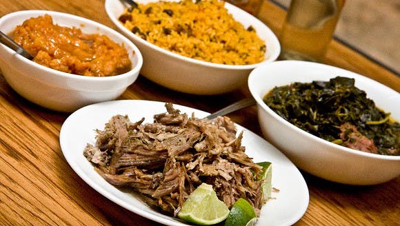
Funny enough, Brasa was also in Man vs Food with Andrew Zimmerman as a guest.
Famous Dave’s is a Midwestern barbecue chain that focuses more on ribs, which isn’t generally considered a Texan specialty. Psycho Suzi’s (a theme restaurant that serves pizza and cocktails) and Brit’s Pub (an English pub with a lawn bowling field) don’t seem very similar, but their cosine similarity scores reflect that.
Donuts
Moving on, let’s find some donuts. Before maple-bacon-cereal-whatever donuts become the craze (thanks for nothing, Portland), my home town was also famous for Round Rock Donuts, a simple and delicious no-nonsense donut shop. And yes, Man vs. Food also did a segment here.

# Round Rock Donuts
retrieve_recommendations(228)
| cosineSimilarity | Name | City | state | Location | category | rating | selfRating | |
|---|---|---|---|---|---|---|---|---|
| 228 | 1.000000 | Round Rock Donuts | Round Rock | TX | Austin, TX | Coffee Shop | 9.4 | 10.0 |
| 825 | 0.962594 | Glam Doll Donuts | Minneapolis | MN | Minneapolis, MN | Donut Shop | 9.1 | 2.0 |
| 670 | 0.873971 | Granny Donuts | West Saint Paul | MN | Minneapolis, MN | Donut Shop | 7.5 | NaN |
| 827 | 0.866257 | YoYo Donuts and Coffee Bar | Hopkins | MN | Minneapolis, MN | Donut Shop | 8.4 | 2.0 |
| 826 | 0.862637 | Bogart's Doughnut Co. | Minneapolis | MN | Minneapolis, MN | Donut Shop | 7.7 | NaN |
| 830 | 0.847556 | Mojo Monkey Donuts | Saint Paul | MN | Minneapolis, MN | Donut Shop | 8.3 | 2.0 |
Sadly, a lot of the most similar places our results returned were places I’ve tried and didn’t like. For some reason, the donuts at most places up here are usually cold, cake-based, and covered in kitschy stuff like bacon. However, Granny donuts looks like it could be promising, as does Bogart’s:

Tacos
This is another Austin specialty that likely won’t give promising results, but let’s try it anyway.
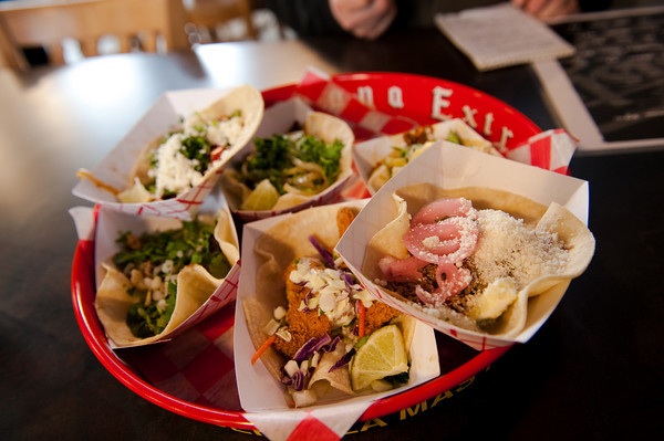
Tacodeli is my personal favorite taco place in Austin (yes, it’s better than Torchy’s), and they’re a little different than the traditional taco (corn tortilla, meat, onions, cilantro, and lime that you might find at traditional Mexican taquerias). They’re typically on flour tortillas, and diversify their flavor profiles and toppings:
/cdn.vox-cdn.com/uploads/chorus_image/image/53151105/16112919_10154883686894449_6136333774221690944_o.0.0.jpg)
# Tacodeli
retrieve_recommendations(420)
| cosineSimilarity | Name | City | state | Location | category | rating | selfRating | |
|---|---|---|---|---|---|---|---|---|
| 420 | 1.000000 | Tacodeli | Austin | TX | Austin, TX | Taco Place | 9.2 | 10.0 |
| 986 | 0.869268 | Rusty Taco | Minneapolis | MN | Minneapolis, MN | Taco Place | 8.1 | 4.0 |
| 849 | 0.826003 | Taco Taxi | Minneapolis | MN | Minneapolis, MN | Taco Place | 8.4 | NaN |
| 1114 | 0.270148 | Psycho Suzi's Motor Lounge & Tiki Garden | Minneapolis | MN | Minneapolis, MN | Theme Restaurant | 8.5 | 2.0 |
| 579 | 0.259052 | Hell's Kitchen | Minneapolis | MN | Minneapolis, MN | American Restaurant | 8.9 | 4.0 |
| 838 | 0.256581 | Brit's Pub & Eating Establishment | Minneapolis | MN | Minneapolis, MN | English Restaurant | 8.8 | NaN |
It looks like there’s a pretty sharp drop-off in cosine similarity after our second recommendation (which makes sense when you look at the ratio of taco places in Austin vs. Minneapolis from when we pulled our data), so I’m going to discard the bottom three. I’m surprised again that Psycho Suzi’s and Brit’s Pub made a second appearance since neither of them serve tacos, but I won’t into that too much since their cosine similarity is really low.
I have tried Rusty Taco, and it does seem a lot like Tacodeli. They even sell breakfast tacos, which is a very Texan thing that can be rare in the rest of the country. The primary difference is in the diversity and freshness of ingredients, and subsequently for me, taste:
Taco Taxi looks like it could be promising, but they appear to be more of a traditional taqueria (delicious but dissimilar). To be fair, taquerias have had the best tacos I’ve found up here (though most of them aren’t included in this list because they were outside of the search range).
Burritos
I’m not actually going to run our similarity function for this part because the burrito place back home actually disappeared from our data pulling query in between me originally running this and finally having time to annotate everything and write this post. However, I wanted to include it because it was one of my other field tests.
Cabo Bob’s is my favorite burrito place back home, and they made it to the semi-finals in the 538 best burrito in America search losing to the overall champion. To anyone not familiar with non-chain burrito restaurants, they are similar to Chipotle, but are usually higher quality.

El Burrito Mercado returned as highly similar, so we tried it. It’s tucked in the back of a mercado, and has both a sit-down section as well as a lunch line similar to Cabo Bob’s. We decided to go for the sit-down section since we had come from the opposite side of the metropolitan area, so the experience was a little different. My burrito was more of a traditional Mexican burrito (as opposed to Tex-Mex), but it was still pretty darn good.

Indian
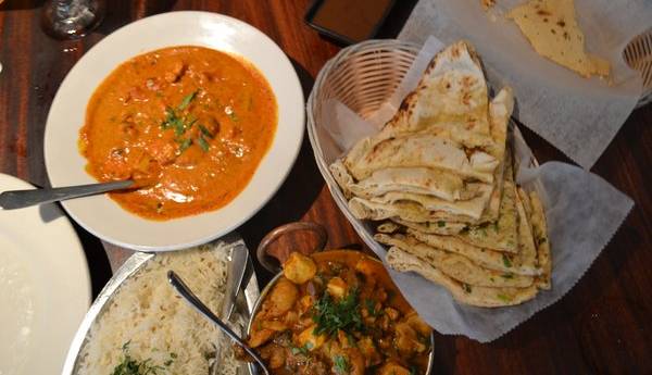
Next up is the the Clay Pit, a contemporary Indian restaurant in Austin. They focus mostly on curry dishes with naan, though some of my friends from grad school can tell you that India has way more cuisine diversity than curry dishes.
# Clay Pit
retrieve_recommendations(338, 8)
| cosineSimilarity | Name | City | state | Location | category | rating | selfRating | |
|---|---|---|---|---|---|---|---|---|
| 338 | 1.000000 | Clay Pit Contemporary Indian Cuisine | Austin | TX | Austin, TX | Indian Restaurant | 8.9 | 9.0 |
| 904 | 0.874870 | India Palace | Saint Paul | MN | Minneapolis, MN | Indian Restaurant | 7.9 | NaN |
| 909 | 0.853726 | Darbar India Grill | Minneapolis | MN | Minneapolis, MN | Indian Restaurant | 7.7 | NaN |
| 905 | 0.848635 | Dancing Ganesha | Minneapolis | MN | Minneapolis, MN | Indian Restaurant | 7.3 | NaN |
| 916 | 0.847020 | Gandhi Mahal | Minneapolis | MN | Minneapolis, MN | Indian Restaurant | 8.0 | NaN |
| 917 | 0.845153 | Best of India Indian Restaurant | Saint Louis Park | MN | Minneapolis, MN | Indian Restaurant | 7.6 | NaN |
| 906 | 0.837536 | Gorkha Palace | Minneapolis | MN | Minneapolis, MN | Indian Restaurant | 9.0 | NaN |
| 912 | 0.834911 | India House | Saint Paul | MN | Minneapolis, MN | Indian Restaurant | 7.9 | NaN |
| 910 | 0.821674 | Copper Pot Indian Grill | Minneapolis | MN | Minneapolis, MN | Indian Restaurant | 7.3 | NaN |
This was actually the first place I did a field test on. When I originally looked this up, we ended up trying Gorkha Palace since it was the closest one to our house with the best reviews. It has a more expanded offering including Nepali and Tibetan food (though I wasn’t complaining because I love momos. It was delicious, and was very similar to the Clay Pit. We’ll be going back.

French/Bistro
One of our favorite places back home is Blue Dahlia Bistro, a European-style bistro specializing in French fusion. They use a lot of fresh and simple ingredients, and it’s a great place for a date night due to its cozy interior and decorated back patio.

# Blue Dahlia
retrieve_recommendations(124)
| cosineSimilarity | Name | City | state | Location | category | rating | selfRating | |
|---|---|---|---|---|---|---|---|---|
| 124 | 1.000000 | Blue Dahlia Bistro | Austin | TX | Austin, TX | Café | 9.1 | 10.0 |
| 584 | 0.827561 | Wilde Roast Cafe | Minneapolis | MN | Minneapolis, MN | Café | 8.6 | NaN |
| 762 | 0.785928 | Jensen's Cafe | Burnsville | MN | Minneapolis, MN | Café | 8.2 | NaN |
| 741 | 0.781564 | Cafe Latte | Saint Paul | MN | Minneapolis, MN | Café | 9.3 | NaN |
| 759 | 0.777269 | Peoples Organic | Edina | MN | Minneapolis, MN | Café | 8.1 | NaN |
| 686 | 0.772962 | Black Dog, Lowertown | Saint Paul | MN | Minneapolis, MN | Café | 8.6 | NaN |
I think our heavier category weighting is hurting us here since Blue Dahlia is classified as a café. Most of the recommendations focus on American food (remember, American food is king in Minneapolis), but I’m guessing the Wilde Roast Cafe was listed as the most similar restaurant due to the similarly cozy interior and various espresso drinks they offer. I’ve been to the Wilde Roast before beginning this project, and I can tell you that the food is completely different.

Coffee
Speaking of coffee, let’s wrap this up with coffee recommendations. I still have a lot of places to find matches for, but since I did this project as a poor graduate student, most of them would be “that looks promising, but I haven’t tried it yet”.
Sadly, a lot of my favorite coffee shops from in and around Austin didn’t show up since Starbucks took up most of the space when searching for coffee places (remember, we’re limited to 50 results per category). We ended up with Mozart’s:

and the Coffee Bean & Tea Leaf:

I ran the results for Mozart’s and didn’t get anything too similar back. To be fair, there aren’t any coffee shops on a river up here, and I’m sure most comments for Mozart’s are about the view.
Let’s go with The Coffee Bean & Tea Leaf instead. It’s actually a small chain out of California that is, in my opinion, tastier than Starbucks.
# Coffee Bean & Tea Leaf
retrieve_recommendations(558)
| cosineSimilarity | Name | City | state | Location | category | rating | selfRating | |
|---|---|---|---|---|---|---|---|---|
| 558 | 1.000000 | The Coffee Bean & Tea Leaf | Austin | TX | Austin, TX | Coffee Shop | 8.1 | 8.0 |
| 742 | 0.811790 | Five Watt Coffee | Minneapolis | MN | Minneapolis, MN | Coffee Shop | 8.9 | NaN |
| 747 | 0.805479 | Dunn Bros Coffee | Minneapolis | MN | Minneapolis, MN | Coffee Shop | 7.9 | NaN |
| 757 | 0.797197 | Caribou Coffee | Savage | MN | Minneapolis, MN | Coffee Shop | 7.7 | NaN |
| 760 | 0.791427 | Dunn Bros Coffee | Minneapolis | MN | Minneapolis, MN | Coffee Shop | 7.1 | NaN |
| 778 | 0.790609 | Starbucks | Bloomington | MN | Minneapolis, MN | Coffee Shop | 8.0 | NaN |
These are perfectly logical results. Caribou is a chain popular in the Midwest (I also describe it as ‘like Starbucks but better’ to friends back home), and Dunn Bros is similar, but specific to Minnesota.
This chart from an article on FlowingData helps describe why I think these results make so much sense:

As for my verdict on Caribou, I actually like it better than the Coffee Bean and Tea Leaf. In fact, I actually have a gift card for them in my wallet right now. There also used to be a location for the Coffee Bean and Tea Leaf up here, but they closed it down shortly after I moved here (just like all of the Minnesotan Schlotzsky’s locations…I’m still mad about that).
Summary
Like any other tool, this method isn’t perfect for every application, but it can work if we use it effectively. While there is room for improvement, I am pleased with how it has been working for me so far.
I’m going to continue to use this when we can’t decide on a restaurant and feeling homesick, and will likely update this post in the future with either more places I try out or when I move to a new city in the future. In the meantime, I hope you enjoyed reading, and feel free to use my code (here is the github link) to try it out for your own purposes.
Happy eating!